Contact Us
LTI Optics is always striving to improve customer support and provide you timely product updates and information to increase your productivity. If you have questions about your software, we invite you to review the sections above and check for new product downloads.
You may email support inquiries to us at the follow address: 
Should you need to call us, our support hours are 8 AM - 5 PM MST. Please review the technical support policy. Our technical support staff can be reached at 720-891-0030.
Installation and Licensing
Requirements
It's all about speed and memory. Since Photopia is processor intensive, you'll experience best results with a fast processor. We would also recommend a multi processor / core machine since Photopia is multithreaded. You'll need enough memory so that the model and raytrace can be stored in memory and not paged to the hard drive. For most models, 2 GB should be sufficient. You'll also want to have a graphics card that supports OpenGL.
Minimum System Requirements:
- Windows 7 Service Pack 1 or greater, Windows 8 or Windows 10, 32 or 64bit
- 4GB of RAM
MacOS:
In order to run Photopia in MacOS, it will need to be under Windows 7 SP1 or greater. You can do this either with BootCamp or under a virtual solution like VMWare Fusion or Parallels.
My Photopia | Online Licensing
Beginning with Photopia 2020.1 released August 2020, Photopia uses a new online licensing system. There are no more Site Codes, Authorization Keys, or License Servers to maintain.
Working Online and Offline
When must you login with your email and password?
- New Installation
- Have not opened Photopia/Solidworks/Reports in the past 30+ days
- Account was locked or password was reset
When must you be online?
- If you haven't opened the software in the last 3 days (default time)
- If your account has restricted offline privileges (not typical)
When can you use Photopia offline?
- If you have had the software open in the last 3 days
- If you currently have the software open
- If you have a checked-out license (coming soon)
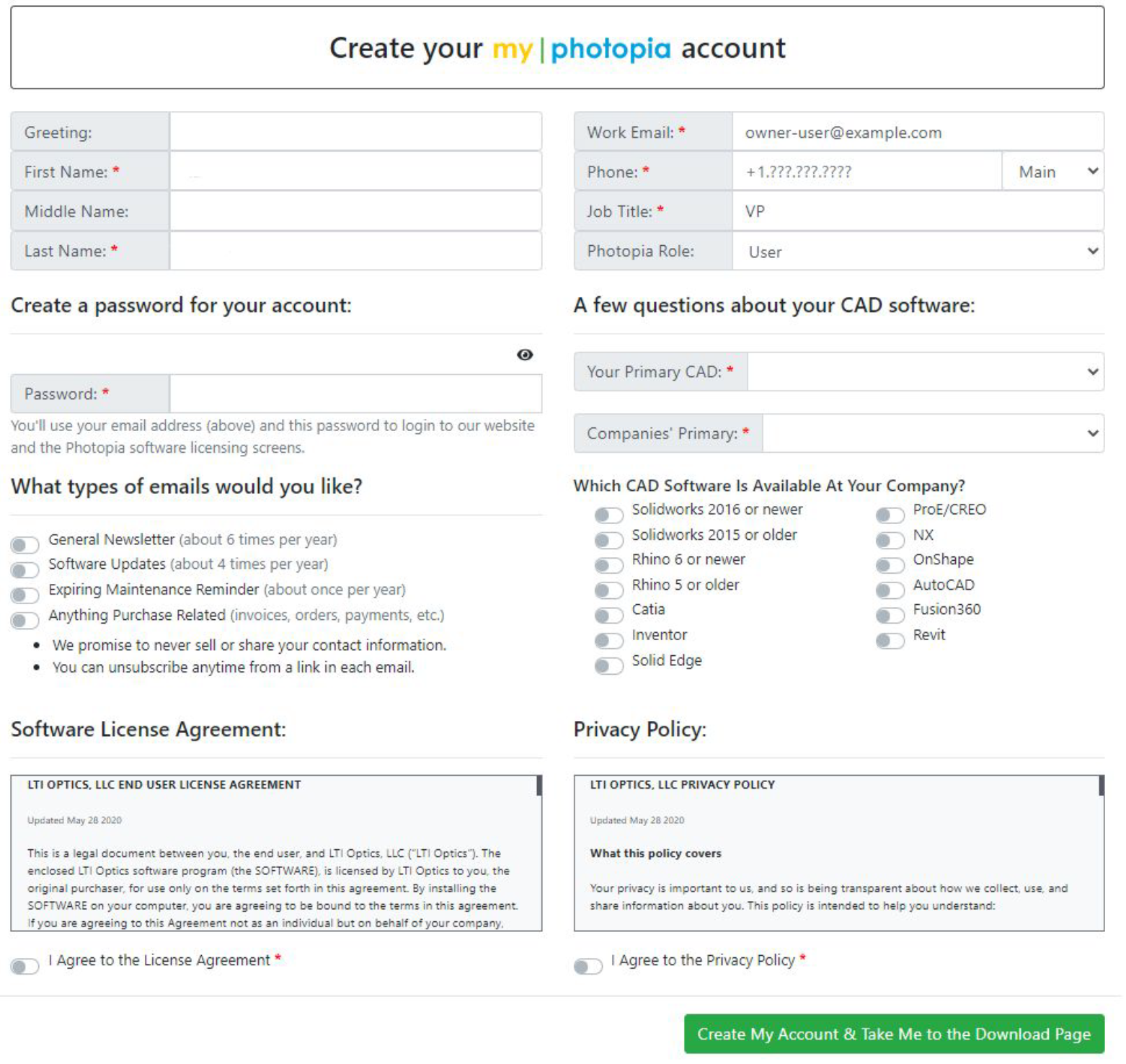
Create your My Photopia Account
LTI Optics will send users an email with a link to setup their online account. All contacts listed for a customer in our database will receive the email invitation to setup their own account.

The user account website will look similar to the one shown below. Some information will already be completed, so confirm it is accurate. Required information is marked with an asterisk. Providing details about your CAD software helps us prioritize future development efforts. Click the button to save your updates and go to the page to download the software.
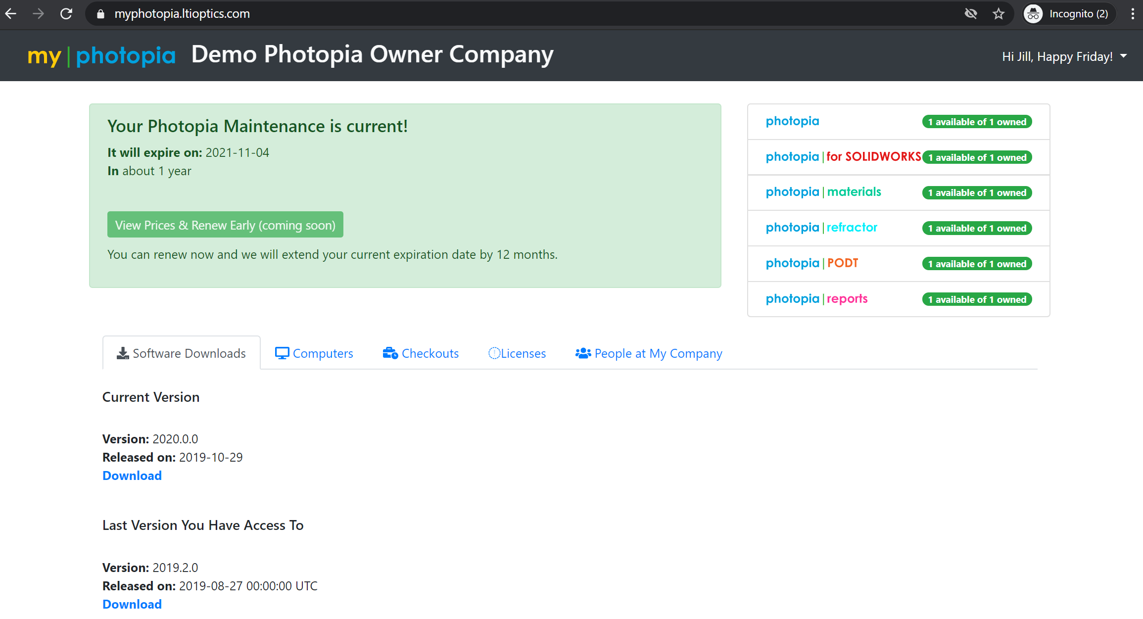
Your My Photopia Page
After completing your profile, you will be directed to your company page. This page includes a range of information, including:
- Software Downloads - Download the latest version you have access to, as well as see the latest update we've released.
- Computer - See which computers have accessed your companies Photopia license.
- Checkouts - See any active license checkouts for your company.
- Licenses - See which licenses you own and the quantity and validity dates.
- People at My Company - See all users at your company.
Software Login
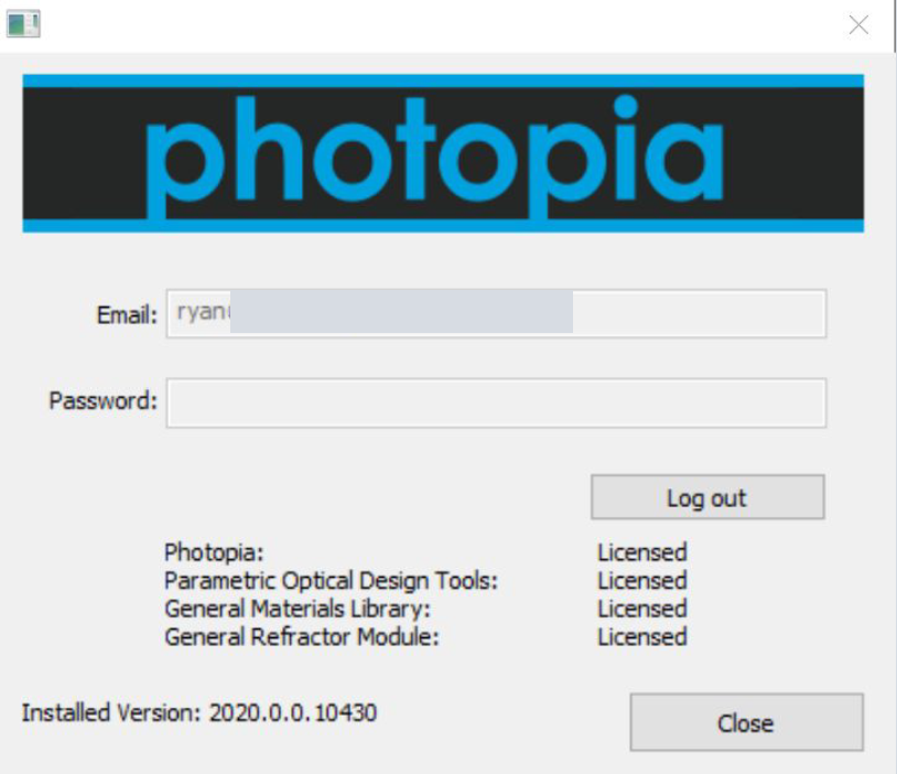
Once you have downloaded and installed Photopia, you can start the program either by opening Photopia, Photopia Reports, or opening SOLIDWORKS with the Photopia Add-In. In Photopia choose License > Login/View and enter the email and password you created earlier. In SOLIDWORKS go to Tools > Photopia > Licensing. In Photopia Reports click the 3 dots and choose Licensing. Once you log in you will see your license status for each module.
Standalone
Switching Users on a computer
If Photopia wasn't installed for All Users, you'll need to re-run the installation for each new user account.
Network
Adding a new network client
You'll need to run the Photopia installation on the client, choosing the Client Installation option. Once installed you'll go to Photopia > License > Authorization, select Client and then enter the servername.
How Photopia Works
Lamps
Photopia Lamp Modeling
Background
Photopia comes with a large library of lamp models for use in optical designs. Sometimes a lamp you may want to use is not in the library. In these cases, you can either construct a lamp model yourself using information in the Photopia User's Guide Appendix B, or have us construct the model for you.
Components in a Lamp Model
Lamp models in the Photopia Library contain 3 basic components: a CAD model, an IES formatted bare lamp photometric file, and luminance information for the source.
The geometry is described in an AutoCAD 2000 formatted DXF file. The model includes all of the physical geometry as well as non-physical geometry such as arc shapes. Materials are assigned to each part of the lamp model, so that the correct interactions occur wen light comes back into contact with the lamp.
The output of the lamp is described in a bare lamp photometric file. This file is created by a lab measurement of the candela distribution and lumen output of each lamp.
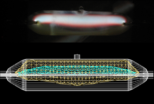
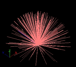
The final part of a lamp model is a description of the luminance properties of the source. For HPS and Metal Halide lamps this means determining the shape and luminance variation of the arc. The image below shows a sample 1500W Metal Halide arc tube with the arc inside, along with the Photopia model of the arc. For fluorescent sources this involves the luminance variation across the surface.
Creating your own Lamp Model
If you are looking for a lamp in the Library and don't find it, you can make your own lamp model. There are instructions for creating lamp models in Appendix B of the Photopia User's Guide, which is available by selecting Help > Documentation in Photopia.
Using an IES file for a lamp
If your luminaire uses LEDs with off the shelf secondary optics from companies such as Ledil, Carclo, Fraen, etc. and if those optics do not interact with other lenses or reflectors in close proximity, then they can be represented using a special set of lamp models in Photopia's library. The special lamp models consist of planar geometry and will emit light in a distribution driven by the IES file you assign to it. The light will be emitted uniformly from the front surface of the lamp geometry. We have created a range of models that can be used for various sized optics. You will see them in the lamp list with names that begin with "LEDLENS..." The rest of the name indicates the geometry of the source, with a single number indicating a diameter. Some of these lamp models also include several copies so you can work with multiple lens types in the same luminaire. In this case, the extra copies have numbers at the end of their name. Some of these models include:
- LEDLENS20MM (This has a round emission area)
- LEDLENS50MM (This has a round emission area)
- LEDLENS75MM (This has a round emission area)
- LEDLENS19x95MM (This has a rectangular emission area for symmetric beams. It is sized for the Ledil Florence product line.)
- LEDLENS95x19MM (This has a rectangular emission area for asymmetric beams where the main throw is perpendicular to the long axis of the lens. It is sized for the Ledil Florence product line.)
To set the lamp model's IES file, just rename your IES file to match the model name you want to use and put it into the following folder: C:\ProgramData\LTI Optics\Library\Lamps
Note that this folder is sometimes hidden by Windows, so if you don't see it in Windows Explorer then change your Folder Options to display all hidden folders and files.
Once you load the lamp into your Photopia project, then you will set its lumens, LED watts and driver watts in the Edit > Design Properties > Lamp screen to define the values appropriate for your LED, its running current, temperature and lens efficiency.
Getting a new lamp in the Library
If you are looking for a lamp in the Library and can't find it, let us know and we'll try to get it in the Library. Lamp manufacturers can have their new products included in the Photopia Library. This is a very beneficial service as your products will be seen by all of our users. You can see more information about adding a new lamp to the Library on this order form.
Raysets
LED Modeling Using Raysets
Overview
Producing accurate simulations of LED based optical systems requires accurate source models. This means the source models must not only produce the correct distribution of light in a far field measurement, they must also produce the correct near field behavior since secondary LED optics are often employed in very close proximity to the LED. Accurate simulations are vital to the design process especially with lens optics commonly used on LEDs given the high cost and long lead times for lens tooling. The data presented in the case studies below is a direct result of the lessons learned by one manufacturer about the importance of simulation accuracy.
What Are Raysets?
Raysets have become a convenient way to model light source behavior, and are commonly provided by LED vendors. A rayset is simply a collection of rays (vectors) that describe the initial emanation of light from a source. Each ray consists of a start point, direction, and magnitude (in lumens). Rayset files are usually provided in multiple formats for compatibility with most optical simulation software.
What Are Raysets Missing?
Raysets are missing one key components of a lamp model, geometry. Raysets only describe the exiting light and do not contain any geometric data about the light source. Since there is no geometric information, there is nothing for the light to interact with if it comes back towards the light source. Some vendors provide 3D cad models as a supplement to their raysets, but this relies on the users to assign appropriate materials to each part of the LED. Additionally, many of these CAD models don't contain enough detail but only describe the bounding volume of the package. This lack of geometry also causes an issue with accurate ray emanation points. Since there is no geometry, the ray emanation points are not coming from geometric locations, but just points in space. The process of combining the 2D images to create raysets does not seem to provide an accurate way to determine correct ray emanation points.
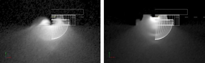
The images below show a cross section of the CREE XR-E LED. The image on the left shows the light field for a rayset based model. The geometry is included only as a reference since the rayset based model doesn't contain any geometric information. The image on the right shows a Photopia lamp model, with the associated geometry. The light field for the Photopia model looks more coherent and seems to match the geometry better than the rayset based model, which seems to indicate light coming directly behind the LED, through the package, which is a physical impossibility.
Using Raysets in Photopia
Since the original beta release, Photopia v3.0 has supported the use of raysets. You can see how to use these in Appendix B of the v3 User's Guide. Photopia uses raysets that end in a .rir extension. Radiant Imaging's ProSource software exports this format natively, and other lamp manufacturers are working on providing this format of their raysets. Our format is identical to the TracePro Binary format, so if you see this format (which ends in a .ray extension) you can use these in Photopia simply by changing the extension to .rir. When you have a .rir rayset, you'll simply import a simple lamp model from the Photopia lamp library, and then in the Property control, choose the rayset by browsing to it. You'll also need to set the appropriate lumen value for the source model.
Rayset Accuracy
Raysets seem to have a good potential of capturing near field photometric data, however, they do have some significant limitations. Their lack of CAD geometry puts the responsibility on the user of the software to import and assign materials in order to achieve an accurate output. Additionally, because the data is compiled from a series of 2D images, raysets often don't contain accurate 3D emanation points. Of the two aspects of lamp modeling, where is the light going and where is it coming from, raysets only accurately adddress where the light is going. Without proper material assignments to the 3D geometry as well as the proper emanation points, photometric simulations can be very inaccurate. Appendix B of the Photopia User's Guide illustrates some of these issues.
In conjunction with Ruud Lighting, we've also done a series of studies that compared simulations with raysets and simulations with Photopia lamp models to measured photometry. We consistently saw very strong correlation between the Photopia lamp models and measured photometry. The match between raysets based models and measured photometry was less consistent. In any application where secondary optics will be placed close to an LED, the Photopia lamp model provides the best correlation. Since these raysets are typically generated from 2D images, they have no way to accurately determine the 3D ray emanation points, which are critical when an optic is placed close to or directly on the LED. Additionally, if an index matching gel is used to join the LED and the optic, raysets provide no way to account for this surface interaction. Case studies are included below as well as in the following papers:
LED Source Modeling Method Evaluations in the November/December 2008 issue of LED Professional Review and LED Source Models in the January/February 2009 issue of LED Journal both cover this study of physical measurements.
These case studies use data collected by BetaLEDTM during the development of their NanoOpticTM LED outdoor area lighting lens optics. The data includes measured luminous intensity distributions along with simulations using both Type 1 and Type 3 source models in Photopia. The optics were measured at Independent Testing Laboratories, Inc. (ITL) in Boulder, Colorado, USA. The simulations used lens geometry that was scanned from the physical as-built parts. This is important since the as-built parts did not always perfectly match the intended design, which removes a potential source of difference between measured and simulated performance.
Case 1: Roadway Type 5 Lens with Index Matching Gel between LED and Lens
The image on the left shows the measured (blue) versus rayset predicted (red) candela plot. The image on the right shows the measured (blue) versus Photopia model predicted (red) candela plot. The rayset based models are called Type 1, the Photopia models are called Type 3 based on the terminology in this paper on lamp modeling.
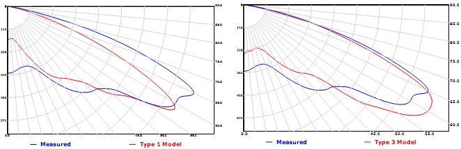
The Photopia (Type 3) model on the right predicts the beam more closely than the rayset (Type 1) model on the left. The image on the right shows that the predicted and measured candela plots trace each other more closely, especially at the higher vertical angles, which are critical in a roadway application. If the simulations are under predicting these values, then the optimization of the optic will be misdirected. The rayset model on the left shows very significant deviations between the high angle light, the angle at which the peak intensity occurs, and the nadir intensity, all of which are main design criteria in a roadway optic.
Case 2: Roadway Type 5 Lens without Index Matching Gel
The differences between the rayset and Photopia model performance are not as great as in Case 1, but the left images below do show an upward shift in the beam angle and significantly more light directly below the luminaire. Accurately predicting the peak vertical angle in the intensity distribution is another critical issue in this type of lens. The right images below show a more accurate overall beam shape and peak beam angles.
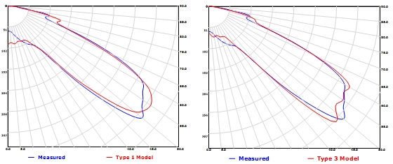
Case 3: Medium Beam Lens with Index Matching Gel
This case illustrates how the differences between the 2 model types remains significant when a gel is used between the LED and lens even in a much narrower beam distribution. The higher intensities seen in the central part of the beam using the Type 1 model on the left result from the extra lumens that were not directed to the higher angles in the distribution where they belonged. The Type 3 model results shown on the right reveal a much closer beam shape at the full range of angles in this distribution.
Summary
The 3 cases presented illustrate that there are significant differences in simulated results depending on the source modeling method used. These results show that a Type 3 model more closely matches the measured performance than the Type 1 model for both wide and medium beam lenses. The differences are greatest when an index matching gel is used between the LED and lens. The main reasons for this are that in addition to the challenge Type 1 models have in creating accurate 3D ray emanation points, all of their digital images showing the luminous view of the source are measured in air. When a gel is used between the LED and the lens, light never exits from the LED primary lens into air so the measurements are inappropriate. Since Type 3 models include the lens geometry, the material can simply be changed to account for the glass / gel interface instead of glass / air.
The 2nd set of data shows that the Type 1 model fairs better when there is no gel, yet it does not outperform the Type 3 model. Wider beam optics are more sensitive than narrower beam optics to exactly how much light is directed onto each part of the lens. As the beam gets narrower, more light is directed to the same angles in the beam and differences in the amount of light sent to each part of the lens between the simulation and physical reality become less important. It should also be noted that other 3D ray emanation point geometry mapping options were tested such as mapping the points to a sphere and the results did not vary significantly from those presented here.
Given a choice between Type 1 and Type 3 source models for the same LED, a Type 3 model will likely produce more accurate results, especially as the beam gets wider. If gels are used between the LED and lens, then Type 1 models should not be used since the measurements on which they are based is not appropriate for this situation.
The simulation data in these case studies was provided by Kurt Wilcox and Chris Strom at Ruud Lighting. ITL in Boulder, Colorado provided the physical measured data for comparison.
Materials
Photopia Materials Library
Background
Our customers rely on Photopia to produce accurate predictive photometry. Having accurate material models is necessary to have accurate output. Photopia includes a library with over 1544 measured materials from most of the major vendors that the lighting industry uses.
Our Measurement Process
LTI Optics uses a custom-built BRDF/BTDF measurement device to accurately characterize the real reflecting/transmitting properties of various materials such as semi-specular aluminum, hammertone, prismatic lenses, perforated diffusers, and many others. The measurements are collected for a wide range of light incidence angles to capture the true scattering nature of real materials (see image below). Photopia uses the measured data in lookup table format and therefore does not attempt to "curve fit" the data into standardized equations that do not model the wide range of scattering effects observed in real materials. The library of measured data also eliminates the need for the user to "guess" at the scattering properties of materials. Customers can also submit proprietary materials for measurement, ensuring the most accurate data possible for their analyses. To create an accurate material model we perform two types of measurements: integrated reflectance/transmittance, and material scattering.
Reflected Intensity Distribution: ALANOD 1165 G3
Adding a Material to the Library
If you're looking for a material that you don't find in the Library, please let us know and we'll work on adding it. Often, you may use a custom material that isn't generally available. We can add this material to a custom library for your company. For information on getting a material in the Library, please see this order form.
Modifying a Material in the Library
You are able to modify the integrated reflectance of reflective materials, the integrated reflectance and transmittance of transmissive materials, and the index of refraction and extinction coefficient of refractive materials. The integrated reflectance and transmittance values can be changed as a function of incidence angle. You can also change the ratio of the light reflected in a specular manner to that scattered by a material and the ratio of the light transmitted in a straight-through manner to that scattered by the material. You cannot change the distribution of the scattered light from materials, however, as this data is measured in our BRDF/BTDF device and stored in binary format. Following are descriptions of the material files:
Reflective Material Files:
Filename.rfl - ASCII file of integrated reflectance values at each incidence angle. Files can contain an arbitrary angle set, so long as 0, 90 and 180 degrees are included. Valid reflectance values range from 0.0 to 1.0.
Filename.brd - Binary file of the BRDF data for a material. This file cannot be modified. A .brd file only 2 bytes in size indicates the material is specular.
Filename.rsc - ASCII file specifying the ratio of the reflected light that is reflected in a specular manner. Note that these are not the specular reflectance values, but the fraction of the reflected light that is specular at each angle. To derive specular reflectance from these values, multiply these values by the reflectance at each incidence angle. Valid values range from 0.0 to 1.0. This file may or may not be associated with a material. A data byte indicating whether or not the material has a specular reflectance component is contained in the .brd file.
Transmissive Material Files (includes reflective files above, plus the following):
Filename.trn - ASCII file of integrated transmittance values at each incidence angle. Files can contain an arbitrary angle set, so long as 0, 90 and 180 degrees are included. Valid transmittance values range from 0.0 to 1.0.
Filename.btd - Binary file of the BTDF data for a material. This file cannot be modified. A .btd file only 2 bytes in size indicates the material is clear or image-preserving.
Filename.tsc - ASCII file specifying the ratio of the transmitted light that is transmitted in a straight-through manner. Note that these are not the straight-through transmittance values, but the fraction of the transmitted light that passes through un-scattered at each angle. To derive straight-through transmittance from these values, multiply these values by the transmittance at each incidence angle. Valid values range from 0.0 to 1.0. This file may or may not be associated with a material. A data byte indicating whether or not the material has a straight-through transmittance component is contained in the .btd file.
Refractor Materials Files:
Filename.rfc - ASCII file containing 3 values: the index of refraction of the outside medium (usually assumed to be air at 1.0), the index of refraction of the material averaged over the visible spectrum, and the extinction coefficient in units of inches. Note that the extinction coefficient is applied in the equation: Trans = e^(k*L), where e is the exponential (2.71Ö), k is the extinction coefficient, and L is the distance the ray travels in the material in inches. Thus, k is a value per inch.
To Modify Material Files:
You can modify any of the ASCII files described above with a text editor such as Notepad. If you want to create a new version of a file without changing the original copy, then follow the specific instructions below:
- Go to the \Photopia\Lib subdirectory.
- Find a material that has all of the same general characteristics as the new material you wish to create. For example, pick PAINT001 if you want a reflective material that has a specular component.
- Copy all of the files for the original material to files with a new filename of your choice. Keep the filename prefix to 8 characters or less.
- Modify the data in the files as you require.
- Add a reference to your new material in either the Reflect.lib, Transmit.lib, or Refract.lib file, depending on if your file is reflective, transmissive, or refractive, respectively. These files are ASCII files. Open the proper file in Notepad or another ASCII file editor and copy the last line in the file to a new line. Then modify the data as you require. There are 5 entries on each line, with each piece of data separated by a TAB character. In order, the data is: manufacturer, designation, description, value (either nadir reflectance, nadir transmittance, or index of refraction), and material filename prefix.
- Save and close the .lib file and then your new material should be listed inside Photopia.
Differences Between Refractive and Transmissive Materials
Transmissive surfaces are modeled as infinitely thin surfaces in the CAD model and all optical properties of the physical material are assigned to this surface. When a ray strikes a transmissive surface all of the effects of the thick material are accounted for at this single ray/surface interface. The amount of reflected, transmitted and absorbed light is dictated by the material's .RFL and .TRN files which list the reflectance and transmittance as a function of incidence angle, respectively. The scattering properties for the reflected and transmitted light are dictated by the BRDF and BTDF data, respectively. The "front" side of the material always has reflectance and transmittance properties and the "back" side has data on only some of the materials in the library. Examples of transmissive materials are clear glass and plastics, white translucent materials, isotropic* prismatic lenses and isotropic perforated materials.
Refractive surfaces model the entire volume of a lens including the inside, outside and side surfaces. When a ray strikes a refractor surface from the "outside" (from the air, for example), it is partially reflected and refracted according to Fresnel's Equations and Snell's Law of Refraction, respectively. Light is also absorbed within the material according to the path length within the material and the material's extinction coefficient. Once rays have entered into a refractor material such as glass, Photopia searches for intersections with other refractor surfaces on all refractor layers in the model. Once an intersection is found, the ray is either partially internally reflected and partially refracted out or it is Totally Internally Reflected (TIR) back into the material, depending on the incidence angle.
Clear lenses can be modeled with either Transmissive or Refractive surfaces. Transmissive surfaces will result in a faster analysis. If the lens is curved, then only the inside surface of the true lens shape should be modeled if making it a Transmissive surface. If the curvature and thickness of the clear lens are such that there might be some refractive effects, then it should be modeled as a Refractor using its true geometry and thickness.
*Isotropic materials are those for which their orientation within the plane of the material is not important. For example, a flat sheet of translucent white plastic can be rotated within the plane of the material and the scattering of the incident light will be unaffected. If a material such as a plastic lens with extruded linear prisms was rotated there would be a significant difference between the scattered light patterns. The effects of the prisms on the light are different depending on whether the light strikes the prisms from within a plane that is parallel, perpendicular or some other orientation to them. Such materials are referred to as anisotropic. A perforated material is isotropic if it has round holes in a regular pattern, but it would be anisotropic of it contained linear slots.
When to Use the Solid Model Versions of Transmissive Materials
Transmissive materials use BRDF & BTDF files to characterize how light reflects and transmits when it is incident upon the material. When a ray strikes a transmissive surface in Photopia, the appropriate reaction is applied to the ray using the BRDF & BTDF data. The important point to note is that the measured BRDF & BTDF data takes into account the effects of the full material thickness. So when a ray in Photopia strikes an infinitely thin polygon with a transmissive material assigned to it, the full reaction of the physical material (with a thickness) is accounted for at this single ray/polygon interface.
When a CAD model is constructed as a solid, every part has a thickness. Thus, if a prismatic lens or white diffuser material is drawn as a solid, it will be constructed with the thickness of the physical part. When this model is exported to Photopia via a STL file it imports as a mesh of polygons that cover the surface of the original solid model. If a transmissive material is assigned to the mesh that models this lens, then a ray will encounter 2 surfaces when passing through the material model. Since the full effect of the material is accounted for at the first ray/surface interaction, it will then be accounted for twice if the ray then strikes a second surface of the lens.
To avoid this problem, we have made special versions of the transmissive materials where the second surface is ignored in such a case. These are the Solid Model versions of the transmissive materials and they should be used when the CAD model was constructed as a solid model. Note however, that the Solid Model versions of the materials only produce the proper effect if all of the surfaces of the lens model are oriented so that their "front" side is facing to the outside of the part. Thus, if the part is on a layer with a color of white, then the part should be rendered as white from all points of view when viewed in the Show Surface Orientation model in Photopia. This is important because the way that the Solid Model materials work is to have the reaction on the "back" side of the material be perfectly transmissive. So when the ray encounters the second surface of a lens model, it strikes the "back" side and is allowed to pass directly through with no losses or scattering.
One significant consequence of this is that it prohibits (or at least limits) the use of materials with different properties on each side. Materials that have a textured surface on one side and a smooth finish on the another, for example, can be properly modeled with a single, infinitely thin surface in Photopia since we can assign unique BRDF & BTDF data to each side of the material. But in the case of Solid Model materials, the "back" side must be set to be perfectly clear, so this flexibility is lost. This is why all of the Solid Model materials in the library are for materials that are the same (or mostly the same) on both sides. If you have a need for another material to be made into a Solid Model material, then contact us about making a new material for you. It is possible to make Solid Model materials for materials that are different on each side as long as light is only incident onto one side of the lens in the luminaire model.
Volumetric Scattering
Background
Beginning with Photopia 2017, Photopia and Photopia for SOLIDWORKS support volumetric scattering refractive materials. This is for materials which scatter light within their volume, usually via pigment or diffusion particles. These are a special class of Refractive materials, and as such require the General Refractor Module or Photopia Premium. Volumetric scattering can also be used along with spectral material properties to model phosphor particles suspended in a clear material.
Description
Photopia uses a specific XML formatted file for defining the material properties. For Volumetric Scattering, the scattering is described by the Beer-Lambert Law. Photopia accounts for the extinction coefficient within the clear base material, the scattering coefficient (likelihood to scatter), the absorption of the scatter reaction, as well as the distribution and energy conversion of the scatter reaction.
Full details are provided in this Volumetric Scattering Documentation.
Spectral Materials
Background
With Photopia 2015, we introduced the ability to set spectral properties for materials. For spectral materials to function, a raytrace must be set as an SPD raytrace. You must also have appropriate .material, .spdrfc, .spdrfl, .spdtrn, and .spdmatrix files.
.material file
Each spectral material must have a .material file. This is an XML based file that tells Photopia what files contain the data for the given material.
- the label “id” must have “matlname (matl type)
- depending on the material type, lines for the brd,btd,rfl,trn,rfc,spdrfc,spdrfl,spdtrn can be included
- for refractive materials, if brd/btd/rfl/trn files are included then the material will refract but use the scattering data (no more flags in the rfc file)
- the individual file names do not matter, however their extensions must be appropriate
.spdrfc file
A .spdrfc file is used for refractors where either the index of refraction or the absorption coefficient or both vary with wavelength.
- name does not need to match .matlname, but must be referenced in the .material file
- 1st row: start wavelength, end wavelength, wavelength increment in nm
- additional rows: outside index of refraction (typically air), inside index of refraction, extinction coefficient
.spdrfl file
The .spdrfl file is the spectral reflectance. The file lists a scale value and then the name of an spdmatrix file for each incident angle.
- name does not need to match matlname, just spdrfl in the .material file
- incidence angle, scale value, spdmatrix filename
- scale value is applied to each value in the matrix

.spdtrn file
The .spdtrn file is the spectral transmittance. The file lists a scale value and then the name of an spdmatrix file for each incident angle.
- name does not need to match matlname, just spdtrn in the .material file
- incidence angle, scale value, spdmatrix filename
- scale value is applied to each value in the matrix
.spdmatrix file
The .spdmatrix file is the spectral material operator file. The format is the same for reflective or transmissive materials. This file can describe something as simple as a paint color or color filter, or it can describe the complex behavior of a phosphor or other wavelength conversion material.
- name does not need to match matlname
- 1st row: start wavelength, end wavelength, wavelength increment in nm
- additional rows: square matrix of wavelength conversion data
- rows are the input nm, columns are the output nm
- for a material that does not convert energy, the matrix will only have values on the diagonal, with zeros in all other locations
- the sum of each row of the matrix must be less than 1 to satisfy conservation of energy
Suggested Raytrace Settings
Since Photopia is a probabilistic based raytracing program, the results get more accurate as more rays are traced. The number of rays that are required to obtain accurate results depends on the level of "resolution" you have specified, in other words, the level of detail in the results. You can view the results such as the candela polar plot and the illuminance plane shaded plot and watch as they vary around their final values with each update as the raytrace proceeds. The default update frequency is 10%, so you see results at 10%, 20% and so on until the raytrace is finished. The least detailed result is the luminaire efficiency (LOR). This is a single number that represents how many lumens exit the luminaire compared to how many lumens were generated by the lamps. The exact direction of the exiting lumens is not critical when determining the efficiency. Thus, you can see that the efficiency changes very little after the first update of the results during the raytrace. The candela distribution requires much more detail to be resolved since Photopia needs to determine exactly how many lumens belong in all of the angular zones of the distribution. The more angles that are specified in the distribution, the smaller the angular zones and thus the more rays it takes to determine the correct proportions of lumens in all zones. The most level of detail is generally required for the illuminance planes. Whereas the angular zones in the candela distribution might be separated by 2.5 or 5 degrees, the small patches in a high-resolution illuminance plane might be separated by fractions of a degree in angular spread. With this general understanding, we make the following recommendations for the Raytrace and Photometric Output settings. Keep in mind that these are only general recommendations and you can vary these values as long as you understand the consequences.
Raytrace & Photometric Output Setting Recommendations
| Applications | Photometry Type | # of Rays - Initial Evaluation | # of Rays - Final Evaluation | # of Reflections - No Lens | # of Reflections - With Lens | Vertical Angle Increment | Horizontal Angle Increment |
|---|---|---|---|---|---|---|---|
| Wide Beam | C | 500,000 | 5,000,000 | 15 | 25 | 5 | 15 |
| Narrow Beam | C | 500,000 | 5,000,000 | 15 | 25 | 2.5 | 15 |
| Very Narrow Beam | C | 500,000 | 5,000,000 | 15 | 25 | 1 | 15 |
| Roadway or Area Light | C | 2,500,000 | 10,000,000 | 15 | 25 | 5 | 5 or 10 |
| Wide Beam Floodlight | B | 2,500,000 | 10,000,000 | 15 | 25 | 5 | 5 |
| Very Narrow Beam | B | 2,500,000 | 10,000,000 | 15 | 25 | 2.5 | 2.5 |
*Note: When using CFL lamps, we recommend that you turn ON the Lamp Shadow Check option. This options can be left off for most other lamp types. All other raytrace settings can generally be left at their default values.
Energy Units
Photopia 2015 introduced the ability so set the output units to lumens, radiant watts, μmol photons / sec and μmol photons / sec in the 400-700nm range (PAR). This allows the use of Photopia for a wide range of applications from general lighting to agriculture and radiant heating.
Under Setting > Project Settings there is a setting for "Lamp Flux Energy Units". Set this to the units you wish to see for your input and output. You can update your lamp energy values under Edit > Design Properties.
IESX Files
The IESX file contains color/spectral data for each angle in the intensity distribution. This is an XML format file, using a pre-release version of a future IES file format that has been expanded to support luminaire color data. The data in this file can most easily be viewed by opening it in Excel, using a reference style sheet file that tells Excel how to format the data. The style sheet file is named "iesxToText.xslt" and is installed in the following folder on your computer:
C:\Users\Public\Documents\LTI Optics\Photopia\Utilities
Put a copy of this file in the same folder as your IESX file. Then open the IESX file in Excel. At the "Import XML..." pop-up dialog, choose the 2nd option:
"Open the file with the following stylesheet applied (select one):"
It will default to iesxToText.xslt, so keep that option.
Then choose "Delimited" on the Text Import Wizard dialog, then click Next and then choose Comma as the delimiter.
Then click Finish.
The first row in the spreadsheet will include the column labels. If you chose the "Power distribution raytrace" option in Photopia, then the full spectral values will be listed for each angle in the beam at the nm resolution you specified.
CAD Support
SOLIDWORKS
Exporting Drawings from SOLIDWORKS to Photopia
Load your assembly into SOLIDWORKS. Select File > Save As and set the File Type to STL. Select the Options button on the file dialog and use the following settings:
When importing into Photopia you can use the Shift and Ctrl keys to select the entire range of parts you want to import. Photopia will assign layer names for each part using the filenames.
Importing PODT Reflectors from Photopia to SOLIDWORKS.
Inside of Photopia, select the reflector that you want to export. Go to View > Reflector Design from the main menu. On the left side of the screen there is a section titled "Exporting Curve Profile." Click the "Export Curve to Profile" button and select the location where you want to save the DXF drawing. Name the drawing, and select DXF from the drop down menu.
In SOLIDWORKS open your existing assembly or part drawing, or create a new drawing . Select any plane. Choose Insert > DXF/DWG from the main menu. Select the DXF file that you just exported from Photopia. You can then select Next for the Layer Mapping screen. In the following screen, select the "as 3D curves/model" radio button under the CAD view. Then select finish.
Now you can construct the rest of the sketch so that you can extrude or revolve your PODT reflector inside of SOLIDWORKS.
AutoCAD
Importing Lamp Models
AutoCAD 2000 and later versions work such that using the DXFIN command opens a new drawing window instead of importing the geometry directly into the open drawing. The following lists two ways to import lamp models into your existing drawing:
- Using the DXFIN or OPEN command - If you attempt to import a lamp model DXF file into an existing drawing (a non-empty drawing), then AutoCAD 2000 will create a new drawing window into which the lamp model will be placed. This is a consequence of AutoCAD 2000's new Multiple Document Interface (MDI) abilities. You can switch between multiple drawing windows by selecting the drawing name under the Window menu item. The lamp in the new drawing window can be copied by first ensuring that all of the lamp layers are ON, then selecting all of its entities, then copying the lamp to the clipboard via a Ctrl-C or by selecting Copy from the AutoCAD Edit menu. Then switch to your existing drawing and select Paste to Original Coordinates from the Edit menu. NOTE: Be sure that both drawings are in the same UCS so that the lamp is pasted into its proper original orientation.
- Using the INSERT command - The INSERT command now reads both DWG and DXF files. When importing the lamp model this way you can specify the lamp insertion point explicitly in the INSERT dialog or by clicking a point on-screen. If you do not want the lamp to come in as a block, then be sure to the "Explode" checkbox at the bottom of the INSERT dialog. It is recommended that you do Explode the lamp. This will eliminate possible problems with lamp models and blocks. For your convenience, the INSERT command is called when you select the Import Lamp option from the Photopia menu item within AutoCAD. NOTE: The INSERT command does not always scale all parts of the lamp model properly. So if you are applying a scale factor to change the lamp from its original scale in inches to millimeters, for example, then you may have problems. To avoid these problems it is recommended that you do not use the SCALE option in the INSERT dialog and scale as a separate step after the INSERT command is finished.
Solid Models with Photopia 3.1.5 or newer
With Photopia 3.1.5 or better you can directly import solids from AutoCAD. Photopia includes the same meshing options that are available in AutoCAD plus some additional options. You can set Photopia's meshing options by choosing Settings / Application Settings / DXF/DWG. If you have the Triangulation Setting Style set to "Use the Facet Resolution for triangulation settings," then change the Facet Resolution setting to whatever value you require. 10 is the highest value and generally recommended. If you choose "Use triangulation settings" as the Triangulation Setting Style, then you can set the following 3 parameters listed in the dialog to meet your requirements.
Solid models with AutoCAD 2009 or earlier and/or Photopia 3.1.4 or earlier
Before Photopia 3.1.5, Solids must be converted to polyface meshes before being imported. In AutoCAD 2009 and earlier this is done via the 3DSOUT command by following these steps:
- Put each part onto a unique layer. This will facilitate assigning materials in Photopia since materials are assigned to each layer in the model.
- Set the mesh resolution with the FACETRES system variable. The default value of 0.5 is very low and results in a course polygon mesh approximating the shape of your model. We recommend you set the value to a higher level to create a more accurate part shape. If you are using Photopia 1.5, then a value between 5 and 8 is recommended. If you are using Photopia 2.0, then use the maximum setting of 10.
- Export the solids to a 3D Studio files using the 3DSOUT command or by selecting File / Export from main menu and setting 3D Studio as the file type. If you have AutoCAD 2007 or later, please follow these directions to enable the 3DSOUT command. Keep the default settings on the 3D Studio File Export Options screen. Note: If the mesh contains too many vertices, then AutoCAD will not export the part. The 3DSOUT command will give an error message if this occurs. If you encounter this problem, then try one of the following options:
Reduce the FACETRES variable to a lower value and try again. If the 3DSOUT command continues to fail or if the facet resolution is not acceptable at the level AutoCAD will support, then try the next option.
Use the EXPLODE command on the solid to convert it to a set of regions and/or bodies. Then create several new layers and put a portion of the regions and bodies onto each of the new layers. Now try and export the set of regions and bodies from each layer individually using the 3DSOUT command. If it still fails, then reduce the amount of geometry on each layer until it succeeds - Import the 3D Studio file into a new AutoCAD drawing using the 3DSIN command or by selecting Insert / 3D Studio from the main menu. Click the Add All button in the Available Objects section of the Import 3D Studio File Options screen and keep the rest of the settings at their default values.
- Save the meshed parts to a 2000 DWG file. This .DWG file can then be imported into Photopia.
3DSOUT Command
For AutoCAD 2007-2009, the 3DSOUT command which is used to create .3ds files from AutoCAD drawings, was removed. This command was widely used to convert solids within AutoCAD to faces. AutoCAD has released a patch which re-enables the 3DSOUT command in AutoCAD 2007-2009. Follow these directions to install and use the command:
- Download the 32-bit and 64-bit version of the patch, save it to a temporary location, and unzip the folder.
- Double click the 3dsout32bit_enu.exe or 3dsout64bit_enu.exe to run the installation.
- Accept the license agreeement.
- Enter the location of the program folder for which you want to use the 3DSOUT command (for example, C:\Program Files\AutoCAD2007).
- Open AutoCAD and type "appload" at the command prompt.
- In the Load/Unload Application dialog box, navigate to the folder where you installed the Ac3Dsout.arx file and select it and click Load and Close.
- Use the 3dsout command like you normally would, by typing 3DSOUT at the command link and then selecting the objects to export.
AutoCAD 2010 and later no longer support the 3DSOUT command and the program referenced above cannot be used. However, since Photopia V3.1.5 and later import solids directly, there is no longer a need to convert solids to meshes in AutoCAD. Photopia includes the same meshing options that were previously available in AutoCAD plus some additional options. You can set Photopia's meshing options by choosing Settings / Application Settings / DXF/DWG. If you have the Triangulation Setting Style set to "Use the Facet Resolution for triangulation settings," then change the Facet Resolution setting to whatever value you require. 10 is the highest value and generally recommended. If you choose "Use triangulation settings" as the Triangulation Setting Style, then you can set the following 3 parameters listed in the dialog to meet your requirements.
*This information was taken from the AutoCAD website and the exe files are from AutoCAD. LTI Optics, LLC makes no guarantees.
Converting 2D Part Drawings to 3D Models
- Open the 2D drawing containing the reflector profile. The following steps assume that the 2D geometry is constructed in the XY plane of AutoCAD's World Coordinate System (WCS).
- Define new layers in AutoCAD for 2D profiles and 3D surfaces for the various luminaire components, i.e. Profile-Main, Refl-Main, Profile-Lens, Tran-Lens, etc.
- Delete extraneous geometry so that only the essential geometry remains that is required to make the 3D surfaces of the various luminaire parts, i.e. lines or polylines describing the reflector profile, lens profile and lamp holder locations.
- Change the properties of the 2D entities so that they reside on the appropriate layers just created in AutoCAD, i.e. put the main reflector profile on layer Profile-Main.
- Move the entities (lines, arcs, etc.) that comprise the 2D profiles of the luminaire components so that the center of the luminaire opening is located at (0,0,0) in AutoCAD's WCS.
- Rotate the 2D profiles of the luminaire components so that the reflector opening is oriented toward the -Y axis if the luminaire produces downward directed light or toward the +Y axis if the luminaire produces upward directed light.
- Change the view to an isometric view that allows the geometry to be seen in 3D. The "SE Isometric" view is a good choice. This can be obtained from the View toolbar or from the menu (R14: View - 3D Viewpoint - SE Isometric) or (2000-2002: View - 3D Views - SE Isometric)
- From the main menu, select Modify - 3D Operation - Rotate 3D to rotate the 2D profiles for the luminaire geometry so that it is tilted up into the Front view (the Front view is in the world XZ plane). This is done by rotating the geometry +90° about the world X axis.
- If the reflector is comprised of linear extrusions, then create the appropriate "direction vectors" in preparation for the "TABSURF" command. To make a direction vector, draw a "Line" entity the proper length and direction. Then make the appropriate 3D geometry layer current, for example Refl-Main, so that the new polyline mesh created by the TABSURF command will be created on the appropriate layer. After the mesh is created, it needs to be moved half its length so that it is centered about the profile used to create it. Note, all Line entities should be converted to Polylines using the "PEDIT" command. Also note that all Arc entities will be subdivided along their profile according to the SURFTAB1 setting.
- If the reflector is comprised of circular components, then create the appropriate "axis of revolution" in preparation for the "REVSURF" command. To make an axis of revolution, draw a "Line" entity at the proper location and in the proper direction. Then make the appropriate 3D geometry layer current, for example Refl-Main, so that the new polyline mesh created by the REVSURF command will be created on the appropriate layer. The revolved surface will have an azimuthal resolution defined by the SURFTAB1 setting. Note, all Line entities should be converted to Polylines using the "PEDIT" command. Also note that all Arc entities will be subdivided along their profile according to the SURFTAB2 setting.
- If SAILs are being used to orient surfaces, then make the appropriate SAILs for the 3D reflector surfaces using Lines with a linetype of "DASHED." Remember to put the SAILs onto the same layer as the reflector surfaces to which they are attached.
- If the reflector is a linear extrusion, then construct the end plates using the 3DFACE command. Note that each 3DFACE is 4 sided.
- Import the appropriate lamp model for the design. Rotate, move and scale the lamp as required so that it is placed correctly within the luminaire. Note that all lamp models import with a scale of inches. Thus, if the project is being drawn in millimeters, then the lamp model needs to be scaled by a factor of 25.4. When modifying a lamp model be sure to select all lamp entities at the ends and in the center of the model.
- Copy the lamp model as needed to get the right number of lamps placed within the luminaire. Note that Photopia does not allow lamp models to be mirrored.
- Turn on all lamp, reflector and lens layers for the 3D luminaire parts and turn off all construction and 2D profile layers. Then save the drawing so that it can be imported into Photopia.
Photopia Luminaire Modeling Conventions
- Photopia's coordinate system for photometry - direct light towards -Z, fluorescent lamps along Y axis for quadrilateral symmetry in North America, fluorescent lamps along X axis for bilateral symmetry. Outside North America, the fluorescent lamps should be along the X axis for quadrilateral symmetry and bilateral symmetry.
- Layer naming conventions ("REFL-", "TRAN-", "REFR-")
- SAILs must be DASHED lines
- Importing lamp models into AutoCAD - use the "DXFIN" command
General AutoCAD Reference
AutoCAD has a command line interface similar to Photopia. The following are some basic tools in AutoCAD, with their command alias in square brackets.
Basic Entities:
Surface Creation Tools:
Editing Tools:
Drawing Tools:
Drawing Tasks:
Inventor
Importing Inventor models into Photopia
There are 2 options for importing models from Inventor into Photopia. The first option uses STL files that can be saved directly from Inventor and imported into Photopia. The second option uses SAT files and requires the use of AutoCAD to convert the files to DWG files. The first option is preferred.
1. Export STL files from Inventor Assembly Model:
- Make all required components visible and all non-required components invisible. Components that you do not want in the raytrace do not need to be suppressed, just toggling their visibility is sufficient.
- In the File Menu select Export / Cad Format and choose STL as the file type.
- Click the "Options" button at the bottom of the file dialog.
- Select the appropriate units.
- In the Structure option, choose "one file per instance."
- Set the Resolution as you require.
- See the STL File Considerations section of Chapter 4 of the User’s Guide for additional information on working with STL files
- See the Luminaire Import Wizard section of Chapter 4 of the User’s Guide for a complete description of the import process.
2. Export SAT to AutoCAD and then DWG to Photopia: (requires AutoCAD)
- Import the SAT file into AutoCAD by choosing Insert / ACIS File from the menu.
- Separate the various parts onto different layers once the solid is imported into AutoCAD.
- Save to a DWG file and import that via the Luminaire Import Wizard. Photopia will mesh the solids upon importing them. Under Applications / DXF/DWG, you will see facet resolution settings that determine the smoothness of the meshes made from the solids.
3. Whether you use STL files or a DWG file for your Inventor model, you will need to specify the Photopia lamp model location(s) within your luminaire. This can be done either during the Luminaire Import Wizard or after the luminaire has been completely imported, using Photopia’s internal CAD system.
- The Photopia lamps are all constructed so that their light center is at 0,0,0. Therefore, if you can setup your luminaire assembly so that 0,0,0 is at the lamp center then it will be very easy to locate the Photopia lamp model within your luminaire. If the luminaire uses multiple lamps, then putting 0,0,0 at the center of all lamp location is convenient.
- If it is not convenient to locate 0,0,0 within your model at the lamp center, then we recommend you construct a small cone in your assembly so that the tip of the cone points to the lamp center(s). This way, when the lamp is imported into Photopia and its location is requested, you can use the Osnap to an Endpoint to pick the end of the cone. You can turn off the cone layer within Photopia once the lamps are placed so they will not affect the optical analysis.
Rhino
Converting IGES Files
Rhino will read IGES files of solid or surface based models and convert them to NURBS surface based models. The NURBS surfaces can then be easily converted to polygon meshed based models for use in Photopia, but before they are converted make sure that the parts in the model that use different material finishes are separated onto different layers. This is important since materials are assigned by CAD layer inside Photopia and sometimes all parts are put onto a single layer in IGES files. In this case, you must define a new layer for each part with a different surface finish and then move the parts to their appropriate layer. The steps for this are listed below:
- Define all of the new layers you will require by selecting Edit -> Layers -> Edit Layers. from the main menu.
- Click the New button with the Edit Layers dialog.
- Type in a name that will help you identify the part. We suggest you use the Photopia layer naming convention to make importing the model into Photopia quicker. The Photopia convention specifies that layers begin with either "REFL-," "TRAN-," or "REFR-" to denote them being for reflectors, transmissive surfaces or refractors, respectively. See Chapter 4 in the User's Guide for more details.
- Give the new layer a unique color by clicking on the color patch for that layer.
- To help ease the process of assigning the NURBS surfaces to their appropriate layer, we recommend you turn Off each new layer.
- Once all required layers have been defined, then click OK on the Edit Layers dialog.
- To change the layer of a particular surface, click on one of the boundary lines of that surface. If the boundary you select is shared by 2 surfaces, then Rhino will pop-up a dialog that allows you to toggle or scroll through the alternatives while it highlights them in the CAD view. Pick the surface you desire within this pop-up dialog.
- Once the proper surface has been selected, then choose Edit -> Layers -> Change Object Layer from the main menu and select the layer you want from the dialog displayed.
- If you turned all of the newly created layers off, then the surfaces will be removed from the display as you assign them to their layers. To finish writing out the DXF file see the FAQ on converting NURBS based surface models to polygon meshed based models.
Converting NURBS to Meshes
Rhino contains some very good facilities for creating meshed surface models (or polygon based surface models) from NURBS surfaces or solids. NURBS surfaces can be converted to meshes upon exporting them to DXF files or from within Rhino before the DXF export is started. The easiest method is to convert them at the time the DXF file is written. For greater flexibility on the detail of the mesh however, you can create the meshes for each NURBS surface from within Rhino prior to exporting the DXF file.
Converting NURBS Surfaces Upon Exporting to the DXF file:
- To convert NURBS surfaces to meshes upon exporting to the DXF file, first select the entire model you wish to export. If the model includes Photopia lamps, then be sure to select from the Top view.
- Select File -> Export Selected from the main menu.
- Change the "Files of type" filter at the bottom of the dialog to "AutoCAD DXF," navigate to the proper folder, enter the filename and click the Save button.
- Rhino will then display the AutoCAD Export Options dialog. You can accept the defaults.
- From the Polygon Mesh Options dialog. Select the Detailed Controls. button. Skip to the Polygon Mesh Detailed Options section below.
Converting NURBS Surfaces Within the Drawing Editor:
- To convert NURBS surfaces to a mesh based surface from within the Rhino drawing editor, click on the NURBS surface from which you wish to make a mesh.
- From the Rhino main menu, select Tools -> Polygon Mesh -> From NURBS Object.
- From the Polygon Mesh Options dialog. Select the Detailed Controls. button. Now skip to the Polygon Mesh Detailed Options section below. When finished with that section, return to the next step in this section.
- Once the meshed surfaces are created, you can export them to a DXF file by following the steps listed in the first section. Note that we recommend you put all of the meshes onto unique layers to keep them separate from the original NURBS surfaces. When you create a mesh the NURBS surface still exists and unless you separate the 2 types of surfaces onto different layers they will simply be drawn on top of each other. It is important to separate the 2 when exporting to a DXF file since you need to select the particular surfaces you want to export to DXF. If you select both the mesh and the NURBS surface then you will get twice the number of surfaces you expected in Photopia.
Polygon Mesh Detailed Options:
- Set the "Max Angle" and "Max Aspect Ratio" according to the detailed required for the particular part. We recommend a "Max Aspect Ratio" setting of 100. This is a setting which dictates how long and thin a triangle can become, the aspect ratio referring to the length of the triangle compared to its width. When set to lower levels, a mesh is created which unnecessarily subdivides long flat surfaces which in reality could be described accurately with a single rectangle.
- The "Max Angle" setting refers to the maximum angular difference between the surface normals of adjacent surfaces. When using specular surfaces with relatively small light sources this setting should stay relatively small. We recommend a value of 10 degrees or less. If this value becomes too large, then you will see striations in your light pattern indicative of what the pattern would truly look like if the reflector were really faceted to that degree. If you want a quicker analysis knowing that the striations are not real, then you can set this value to 20 or more. Other general aspects in your light pattern will be accurate. It is common to make course models for early design iterations.
- When the surfaces are black or have a material which scatters the light more, like white paint, hammertone, semi-specular, etc., then you can tolerate less accurate surface orientations and still get accurate analyses. The same holds true when larger light sources are used, such as those which have coated bulbs. In these cases you can increase the "Max Angle" to 20 or 30 degrees. Utilize the Preview button to see if the degree of accuracy introduces any obvious geometric problems.
Importing DXF File Into Photopia
- Start by selected File -> Import Luminaire CAD File from the main menu in Photopia.
- If you use the layer naming convention for Photopia, i.e. REFL-HOUSING, TRAN-LENS, then Photopia will automatically sense the layer types. If you do not use the Photopia layer naming convention, then you need to specify the layer type in the first import screen within Photopia. After all of the layer types have been specified, click Next at the bottom of the dialog.
- The Activate Surfaces screen allows you to specify the surface orientations. Conveniently, the meshes that Rhino makes are such that all polygons of the mesh are oriented the same. Check to see that Photopia has rendered the reflective side of the surfaces in the same color as the layer in Rhino. Note that this is the color that is used on the part when viewed in wireframe mode. We recommend you orient the surfaces of only one layer at a time by clicking on the layer of interest in the list shown in the upper left hand part of the screen. Remember that you can gain full access to all CAD viewing controls by right clicking your mouse in the CAD view window. If the surfaces on a given layer are not rendered in the appropriate color on their reflective or "front" side, then select the "Reverse" Surface Orientation method, then click the "Select All Surfaces" button, then click the "Apply" button. This switches the orientation of all surfaces on the given layer. Once all surfaces have been properly oriented, click Next.
- The last step is to add the lamp(s) to your model. Select the lamp you require from the list within Photopia and use the controls provided to add it and place and orient it. If you need more than one lamp, then add more lamps in the same manner. It is sometimes necessary to change the View Style of the CAD view to "wireframe" to see lamps within the luminaire. Click the Finish button when done.
- You are then prompted to name and specify the location of the project. The default name and location match that of your CAD file. Note that the Photopia project is comprised of a series of files all sharing the same filename prefix.
SolidEdge
Exporting Files to Photopia
There are three options for importing Solid Edge models.
Option #1
If you have AutoCAD in addition to Solid Edge, then you can convert the Solid Edge model to a 3D DWG file by following these steps:
- Open your assembly model and save it to an ACIS (SAT) file. Be sure to check the option to include the construction geometry. If you forget this, then AutoCAD will not read the SAT file.
- Import the SAT file into AutoCAD by choosing Insert > ACIS File from the menu.
- Segregate the various solid parts onto different layers in AutoCAD. This will facilitate assigning materials in Photopia since materials are assigned to each layer in the model.
- Set the mesh resolution with the FACETRES system variable. The default value of 0.5 is very low and results in a course polygon mesh approximating the shape of your model. We recommend you set the value to a higher level to create a more accurate part shape. If you are using Photopia 1.5, then a value between 5 and 8 is recommended. If you are using Photopia 2.0 or 3.0, then use the maximum setting of 10.
- Export the solids to a 3D Studio file using the 3DSOUT command or by selecting File > Export from the main menu and setting 3D Studio as the file type. Keep the default settings on the 3D Studio File Export Options screen.
- Import the 3D Studio file into a new AutoCAD drawing using the 3DSIN command or by selecting Insert > 3D Studio from the main menu. Click the Add All button in the Available Objects section of the Import 3D Studio File Options screen and keep the rest of the settings at their default values.
- Save the meshed parts to a DWG file. The DWG file can be imported into Photopia.
- Using this method to convert an Inventor drawing into a meshed model for use in Photopia allows the relationship between the various parts in the assembly to be retained.
- See Chapter 4 of the Userís Guide for additional information on importing DWG files using the Luminaire Import Wizard.
Option #2
Photopia 2.0 and 3.0 accepts solid models in STL format (stereo lithography files). Some CAD programs allow STL files to be exported from the assembly model, while others do not. Exporting from the assembly is preferred since the assembly drawing includes the information that shows how each part is translated with respect to each other. These relationships are retained when the parts are exported from the assembly model. Solid Edge does not, however, allow STL parts to be exported from the assembly model. Therefore, each part needs to be exported from the individual part files. The coordinates of each part are therefore relative to their own coordinate systems. If each part uses an origin (0,0,0) set to some arbitrary reference point on that part, then the parts will not import into Photopia with their correct relative positions. In this case, each part needs to be moved and/or rotated within Photopiaís CAD system to make the proper assembly. The extra work of moving/rotating each part within Photopia can be avoided if all individual part drawings are made with a common origin. For a lighting fixture, the most logical common origin is the center of the lamp, or lamps, if there are several. If this convention is used, then all parts will import into Photopia in their proper relative positions.
Option #3
An alternative to using SAT and STL files is to export the assembly model to an IGES or STEP file and then use a third party translator such as Polytrans or Rhino to convert the IGES or STEP file to a DXF or DWG file. The Photopia FAQ on our website includes full instructions for converting IGES files in Rhino to a DXF file for Photopia.
Importing a PODT Curve from Photopia into Solid Edge
To import a PODT curve from Photopia into Solid Edge, follow these directions:
- Rotate the parametric reflector so that its 2D profile is in the world XY plane in Photopia. Then export the 2D profile as a .DXF file from the Reflector Design View dialog. Note that Photopiaís Rotate command always rotates about the Z axes of the current CPlane. So if you need to rotate a reflector profile from the Front View into the Top View (which is the XY plane), then first set the CPlane to the Right Side View and then rotate -90 degrees about 0,0.
- Start Solid Edge and select File > Open. Then pick .DXF as the file type and specify Normal.dft for the "Draft template." This will open the reflector profile exported from Photopia into a Draft View.
- Select the 2D profile in the draft view and choose the option to edit that individual entity. This will put you into the Draft View Edit mode. (Note: If the Options in the AutoCAD Translation Wizard are set so that the "Map AutoCAD Model Space Entities to a Solid Edge Draft View" option is turned off, then the curve profile will import into the Draft View Edit Mode.)
- Start a new part drawing in Solid Edge using Normal.par as the template.
- Create a sketch and pick the desired plane.
- Go back to the Draft View Edit mode window. Select the curve and then right click your mouse and copy it to the clipboard.
- Then switch back to the Part Sketch window and Paste the curve profile into the sketch.
- Start the Offset command, select the curve, enter an offset distance as the material thickness, and then finish the command being sure to offset it to the "outside" of the curve.
- Then draw line segments to enclose both ends of the profile.
- The part can then be extruded or revolved into a 3D model.
Creo Parametric
Exporting Files to Photopia from ProE
The following directions were taken from Creo Parametric 2001. Directions may vary for other versions, but will be similar.
- Always work in assembly mode. If you have a large assembly (a car, for example) then make your "lighting fixture" a sub-assembly and then assemble it into the main assembly once you are underway.
- Start the assembly with your best 0,0,0 part, usually your reflector or your lamp, as the first component. Try to constrain all other parts to datums, axes, or C Systems based on this part. Never "fix" a component; always fully constrain it.
- Export the parts as STL from within your sub-assembly. Use File > Save As and select .STL.
- Creo Parametric will default the exported filename to the same name as the assembly. Because you need to retain individual parts in Photopia, you will need to delete the assembly name in the file window, and instead enter the name of the first component you wish to export to Photopia. Select OK when done.
- In the STL Export dialogue, select "Include" and pick your first part for export. (If you have several parts which will take the same optical materials you can add these to the selection). Creo Parametric will tell you how many parts you have selected. "Reset" will let you restart the selection process. Next select your coordinate system. Default will use the default CSYS of the assembly. If you created a separate one as your optical center, then make sure to select it.
- Select binary or ASCII, Photopia will read either.
- Select "Allow negative values" as this will keep your parts centered about 0,0,0.
- Select Angle Control and enter a value of 1.
- Select Chord Height and enter 0. Then select the Angle Control window again. The Chord Height will then default to the best available in this part.
- Note that the Chord Height available to you will improve with higher part accuracy settings. It also seems to vary between exports from assemblies and from part mode. This is probably controlled by the accuracy setting of the part versus the assembly file. Call PTC for clarification. Investigate what your settings will look like in Photopia by clicking "Apply" and spinning the resulting image. If you are satisfied, click OK and save the file.
- Repeat this procedure with each individual part.
- Upon import into Photopia, you can select the entire set of files you created. The parts will assemble within Photopia as they did in your Creo Parametric sub-assembly.
STL
Working with STL Files
For specific information about how to export STL files from your CAD software, see the links for your program here.
Exporting STL files from other CAD software
You can find some general instructions for how to export STL files from the following web site: www.vistatek.com/file_stl.htm
Importing STL Files Into Photopia
The best way to import STL files is to select File / Import Luminaire Wizard from the main menu and follow these steps:
- When prompted to select the STL file to import, you should select the entire range of STL files in the file dialog. Photopia will assign default layer names for each part using their filenames. Set the Layer Types for each layer in the list presented in the Import Model dialog by clicking on a layer (or range of layers) and then selecting the appropriate layer type from the drop down list.
- The model needs to be oriented according to Photopia’s photometric coordinate system. The model can quickly be rotated about the X, Y or Z axis using the Rotation feature on the Import Model screen. See the manual or the FAQ on Photometric Conventions for more details on luminaire orientation. Note that you can access all CAD viewing options by right clicking your mouse in the CAD view. Click the Next button when finished with the first screen.
- The surfaces of the STL parts will all be properly oriented by default, so nothing needs to be changed on the Orient Surfaces screen. Click Next.
- Add the desired lamp to the model on the Add Lamp screen. If the lamp needs to be rotated, then that can quickly be done on this screen. If the precise lamp location is not known, then leave the lamp at 0,0,0 and move it in Photopia’s CAD system after completing the import wizard.
- The easiest way to precisely locate lamps is to construct an extra element in the solid model that is a cone, located such that the tip of the cone points to the center of the lamp (or arc tube). After the Luminaire Import Wizard is finished, the lamp can be moved into its precise location using the tip of the cone as a reference point. Make sure the Osnap is turned on in Photopia’s CAD system (toggle the button on the bottom of the screen) and then use the Move command on the lamp model, specifying 0,0,0 as the base point and then picking the tip of the cone as the second point. If multiple lamps are required, then the first lamp can be copied, again using the O Snaps as necessary. See Chapter 4 of the manual for more complete instructions on the Luminaire Import Wizard and the CAD system.
CADKEY
Exporting STL Files to Photopia
If your model is built from solids (bodies), then you can save the parts to STL files. Each part of your assembly needs to be exported to its own STL file. This is because Photopia will put each STL file onto is own layer and materials are assigned to each layer in Photopia. Select the option to save to an STL file from the File menu. We recommend the following export options:
Exporting DXF Files to Photopia
CADKEY can create DXF files and the entities that Photopia requires in DXF files are 3DFACEs or meshes. 3DFACEs are created from CADKEY POLYGONs. You can use whatever means you prefer to create a POLYGON or mesh-based surface model in CADKEY. If you are using SOLIDs to create your reflector surfaces, then you can convert the SOLIDs into POLYGONs by choosing the following from the CADKEY menu: Solids > Application > Convert to Polygons. If there is an equivalent method for creating meshes, then that is preferred by Photopia. Be sure to keep different luminaire parts on different levels in CADKEY so they translate to different "layers" in the DXF file. When importing the DXF file into Photopia you can specify the layer type "Reflective," "Transmissive," etc. for each of your CADKEY levels. You need to separate different parts onto different levels because Photopia assigns luminaire materials on a per "layer" basis.
Microstation
The following information may be helpful to those using Microstation to create 3D models for Photopia. You should first be familiar with the information in Chapter 4 of the Photopia Userís Guide regarding the entity types that Photopia accepts, the layer naming conventions, surface orientation, and luminaire orientation within the global coordinate system.
Acceptable Surface Entities:
Layer (Level) Naming Conventions:
Surface Orientation:
Working With Lamp Models:
Mechanical Desktop
Exporting MDT Files to Photopia
To convert the parametric solids from Mechanical Desktop into polyface meshes, which Photopia accepts, follow these steps:
- Open your assembly model and put each part onto a unique layer. This will facilitate assigning materials in Photopia since materials are assigned to each layer in the model.
- Set the mesh resolution with the FACETRES system variable. The default value of 0.5 is very low and results in a course polygon mesh approximating the shape of your model. We recommend you set the value to a higher level to create a more accurate part shape. If you are using Photopia 1.5, then a value between 5 and 8 is recommended. If you are using Photopia 2.0 or 3.0, then use the maximum setting of 10.
- Export the solids to a 3D Studio file using the 3DSOUT command or by selecting File> Export from main menu and setting 3D Studio as the file type. Keep the default settings on the 3D Studio File Export Options screen.
- Import the 3D Studio file into a new MDT drawing using the 3DSIN command. Click the Add All button in the Available Objects section of the Import 3D Studio File Options screen and keep the rest of the settings at their default values.
- Save the MDT drawing to a DWG file by selecting DWG as the file type in the File > Save As dialog. The DWG file can be imported into Photopia.
Overview
Photopia's CAD System
- Import the 2D drawing containing the reflector profile by selecting File/Import CAD File from the main menu. The following steps assume that the 2D geometry is constructed in the XY plane and therefore imports into the XY plane of Photopia's World Coordinate System (WCS). Photopia uses local coordinate systems called Construction Planes (CPlanes). The current CPlane is indicated in Photopia's CAD system using a red line for the X-axis and a blue line for the Y-axis. The orientation of the WCS is always shown in the lower left corner of the CAD view with the same color conventions, while adding a green Z-axis. The origin (0,0,0) of the CPlane is indicated with a circle and cross hair. See Chapter 4 of the User's Guide for more information about CPlanes. The image below shows the Photopia CAD screen in the Isometric View and illustrates the WCS icon in the lower left corner and the CPlane axes.
- Define new layers in Photopia for 2D profiles and 3D surfaces for the various luminaire components, i.e. Profile-Main, Refl-Main, Profile-Louver, Refl-Louver, Profile-Lens, Tran-Lens, etc.
- Delete extraneous geometry so that only the essential geometry remains that is required to make the 3D surfaces of the various luminaire parts, i.e. lines or polylines describing the reflector profile, lens profile and lamp holder locations. To delete entities in Photopia's CAD system, you can select them individually by clicking on them or select by window or crossing by dragging a window from left to right or right to left, respectively. If all items are linked together in a block, then you can use the EXPLODE command to separate them.
- Change the properties of the 2D entities so that they reside on the appropriate layers just created i.e. put the main reflector profile on layer Profile-Main. To change an entity's layer, select it in the CAD view and change its layer in the property control on the right side of the screen. To de-select an entity, press the Escape key.
- Move the entities (lines, arcs, etc.) that comprise the 2D profiles of the luminaire components so that the center of the luminaire opening is located at (0,0,0) in Photopia's WCS. Type Move or "M" at the command line or choose Modify / Move from the main menu to start the Move command.
- Use the ROTATE command to rotate the 2D profiles of the luminaire components so that the reflector opening is oriented toward the +Y axis, assuming the luminaire produces downward directed light. Rotate it toward the +Y axis if the luminaire produces upward directed light.
- Change the view to an isometric view that allows the geometry to be seen in 3D. This can be done by right clicking your mouse in the CAD view and choosing Standard Views / Isometric View from the pop-up menu.
- The 2D profiles need to be rotated into the Front View (World XZ plane) so that the 3D luminaire is constructed in the right plane. Photopia requires that the beam center for direct luminaires be toward the world -Z axis and the beam center for indirect luminaires be toward the +Z axis. The final step references more information about the required luminaire orientation. Since Photopia does not yet include a 3D rotate command, you will use the standard ROTATE command, which always rotates about the Z-axis of the current CPlane. Therefore, in order to rotate the reflector profile(s) about the world X-axis, the CPlane needs to be set to one of the side views. You will use the Right Side View, which is the world YZ plane. Select Settings / Construction Plane from the main menu, enter "O" for Ortho and "R" for Right. You will see the CPlane axes rotate so that its X-axis aligns with the world Y and its Y-axis aligns with the world Z.
- Select all of the reflector profiles and start the ROTATE command. Enter 0,0 for the base point and 90 degrees for the rotation angle. The reflector should now be rotated into the world XZ plane as shown in the following image.
- If the reflector is comprised of linear extrusions, then you will use the EXTRUDE command. This command extrudes the reflector along the Z-axis of the current CPlane, centering the extrusion about the location of the profile. If the reflector needs to be revolved, then you will use the REVOLVE command. This command revolves the reflector about either the X or Y axis or an arbitrary axis you select. Whether you are extruding or revolving your reflector, you need to change the CPlane to the Front View. So start the CPLANE command, then entering "O" for Ortho and "F" for Front.
- If your reflector profile includes arc entities, then you need to set the resolution of the 3D mesh that will represent the arc. A higher resolution models the shape of the arc more smoothly. For extrusions, enter the SURFTAB1 command and specify the number of segments that will be used to represent it in the mesh. For revolved surfaces, the SURFTAB1 parameter represents the number of segments around the circumference of the mesh, i.e. the smoothness of the circle. The resolution of arc for revolved surfaces is set by the SURFTAB2 parameter.
- If the reflector is a linear extrusion, then construct the end plates using either the POLYGON command or by drawing a horizontal line across the end of the reflector and then using the EXTRUDE command to create a flat plane. Note that POLYGONS in Photopia are triangles, so you will need to draw 2 to make a rectangular end plate. You can use the osnap features to help draw these entities.
- Once the 3D reflectors have been constructed, then you need to ensure they are properly oriented. You can check a surface's orientation by putting the CAD view in the Show Surface Orientation mode. This is an option under View Style on the pop-up menu you get by right clicking in the CAD view. Photopia renders the "front" side of surfaces in the color of its layer and the back side in the opposite color. The reflector materials are applied to the front side of materials and the back side is generally black, so it is important that they are properly oriented. View your model in this mode and orbit around it to confirm the surface orientations. If any of the meshes are oriented incorrectly, then use the Modify / Orient tool to fix them. Select the mesh, then run this tool and enter "R" for reverse.
- Import the appropriate lamp model for the design by selecting File / Import Lamp on the main menu. Enter the location(s) for the lamp. You will be prompted for multiple locations, so just press Enter again at prompt when you are finished entering the locations you require. Use the rotate command in the appropriate CPlane if the lamp needs to be rotated into different orientation than its default.
- See the FAQ topic on Photometric Conventions for more information about the proper orientation of the luminaire, which depends on the type of distribution it creates and your region of the world. Different regions use different standard conventions for photometry.
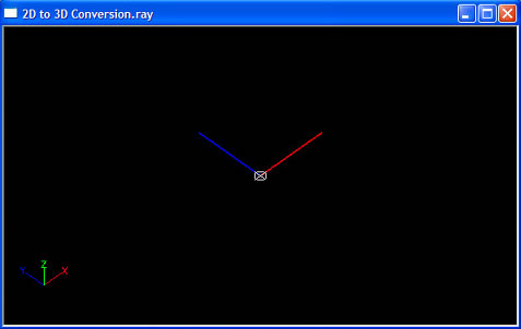
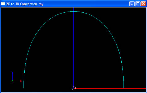
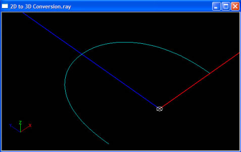
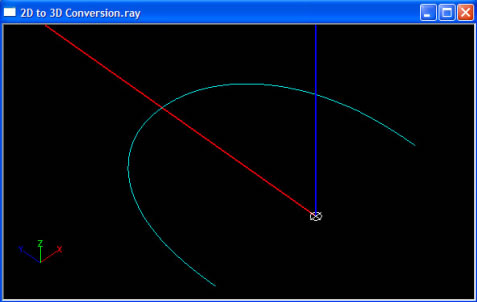
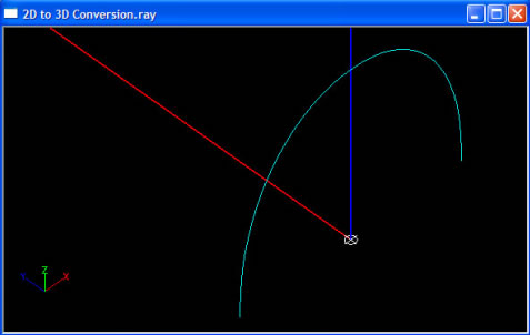
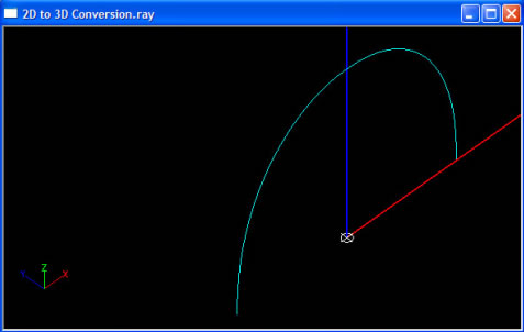
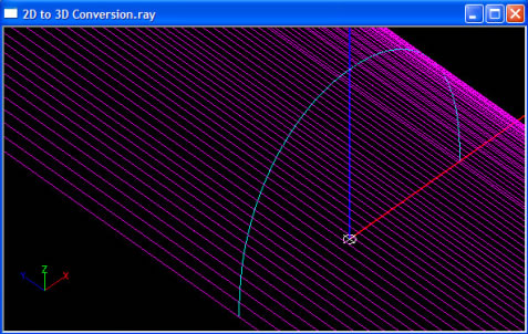
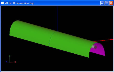
2D to 3D Parts
- Import the 2D drawing containing the reflector profile by selecting File/Import CAD File from the main menu. The following steps assume that the 2D geometry is constructed in the XY plane and therefore imports into the XY plane of Photopia's World Coordinate System (WCS). Photopia uses local coordinate systems called Construction Planes (CPlanes). The current CPlane is indicated in Photopia's CAD system using a red line for the X-axis and a blue line for the Y-axis. The orientation of the WCS is always shown in the lower left corner of the CAD view with the same color conventions, while adding a green Z-axis. The origin (0,0,0) of the CPlane is indicated with a circle and cross hair. See Chapter 4 of the User's Guide for more information about CPlanes. The image below shows the Photopia CAD screen in the Isometric View and illustrates the WCS icon in the lower left corner and the CPlane axes.
- Define new layers in Photopia for 2D profiles and 3D surfaces for the various luminaire components, i.e. Profile-Main, Refl-Main, Profile-Louver, Refl-Louver, Profile-Lens, Tran-Lens, etc.
- Delete extraneous geometry so that only the essential geometry remains that is required to make the 3D surfaces of the various luminaire parts, i.e. lines or polylines describing the reflector profile, lens profile and lamp holder locations. To delete entities in Photopia's CAD system, you can select them individually by clicking on them or select by window or crossing by dragging a window from left to right or right to left, respectively. If all items are linked together in a block, then you can use the EXPLODE command to separate them.
- Change the properties of the 2D entities so that they reside on the appropriate layers just created i.e. put the main reflector profile on layer Profile-Main. To change an entity's layer, select it in the CAD view and change its layer in the property control on the right side of the screen. To de-select an entity, press the Escape key.
- Move the entities (lines, arcs, etc.) that comprise the 2D profiles of the luminaire components so that the center of the luminaire opening is located at (0,0,0) in Photopia's WCS. Type Move or "M" at the command line or choose Modify / Move from the main menu to start the Move command.
- Use the ROTATE command to rotate the 2D profiles of the luminaire components so that the reflector opening is oriented toward the +Y axis, assuming the luminaire produces downward directed light. Rotate it toward the +Y axis if the luminaire produces upward directed light.
- Change the view to an isometric view that allows the geometry to be seen in 3D. This can be done by right clicking your mouse in the CAD view and choosing Standard Views / Isometric View from the pop-up menu.
- The 2D profiles need to be rotated into the Front View (World XZ plane) so that the 3D luminaire is constructed in the right plane. Photopia requires that the beam center for direct luminaires be toward the world -Z axis and the beam center for indirect luminaires be toward the +Z axis. The final step references more information about the required luminaire orientation. Since Photopia does not yet include a 3D rotate command, you will use the standard ROTATE command, which always rotates about the Z-axis of the current CPlane. Therefore, in order to rotate the reflector profile(s) about the world X-axis, the CPlane needs to be set to one of the side views. You will use the Right Side View, which is the world YZ plane. Select Settings / Construction Plane from the main menu, enter "O" for Ortho and "R" for Right. You will see the CPlane axes rotate so that its X-axis aligns with the world Y and its Y-axis aligns with the world Z.
- Select all of the reflector profiles and start the ROTATE command. Enter 0,0 for the base point and 90 degrees for the rotation angle. The reflector should now be rotated into the world XZ plane as shown in the following image.
- If the reflector is comprised of linear extrusions, then you will use the EXTRUDE command. This command extrudes the reflector along the Z-axis of the current CPlane, centering the extrusion about the location of the profile. If the reflector needs to be revolved, then you will use the REVOLVE command. This command revolves the reflector about either the X or Y axis or an arbitrary axis you select. Whether you are extruding or revolving your reflector, you need to change the CPlane to the Front View. So start the CPLANE command, then entering "O" for Ortho and "F" for Front.
- If your reflector profile includes arc entities, then you need to set the resolution of the 3D mesh that will represent the arc. A higher resolution models the shape of the arc more smoothly. For extrusions, enter the SURFTAB1 command and specify the number of segments that will be used to represent it in the mesh. For revolved surfaces, the SURFTAB1 parameter represents the number of segments around the circumference of the mesh, i.e. the smoothness of the circle. The resolution of arc for revolved surfaces is set by the SURFTAB2 parameter.
- If the reflector is a linear extrusion, then construct the end plates using either the POLYGON command or by drawing a horizontal line across the end of the reflector and then using the EXTRUDE command to create a flat plane. Note that POLYGONS in Photopia are triangles, so you will need to draw 2 to make a rectangular end plate. You can use the osnap features to help draw these entities.
- Once the 3D reflectors have been constructed, then you need to ensure they are properly oriented. You can check a surface's orientation by putting the CAD view in the Show Surface Orientation mode. This is an option under View Style on the pop-up menu you get by right clicking in the CAD view. Photopia renders the "front" side of surfaces in the color of its layer and the back side in the opposite color. The reflector materials are applied to the front side of materials and the back side is generally black, so it is important that they are properly oriented. View your model in this mode and orbit around it to confirm the surface orientations. If any of the meshes are oriented incorrectly, then use the Modify / Orient tool to fix them. Select the mesh, then run this tool and enter "R" for reverse.
- Import the appropriate lamp model for the design by selecting File / Import Lamp on the main menu. Enter the location(s) for the lamp. You will be prompted for multiple locations, so just press Enter again at prompt when you are finished entering the locations you require. Use the rotate command in the appropriate CPlane if the lamp needs to be rotated into different orientation than its default.
- See the FAQ topic on Photometric Conventions for more information about the proper orientation of the luminaire, which depends on the type of distribution it creates and your region of the world. Different regions use different standard conventions for photometry.
Photometry
Conventions
Having the correct Photometric Settings is critical to obtaining accurate results from Photopia. When you send a product for testing, the laboratory often determines the correct photometric angles, but when you are running Photopia it is something you must always be aware of. The angle sets are often broken down to vertical and horizontal angles, described below.
Vertical Angles
Vertical photometric angles go from directly below the fixture at 0 degrees to directly above at 180 degrees. The vertical angles that you choose are governed by the vertical distribution of your product. See the table below for information on the correct choice of vertical angles.
| Direct | Indirect | Direct/Indirect | |
|---|---|---|---|
| Distribution | Light Directed Downward | Light Directed Upward | Light Directed Upward and Downward |
| Orientation | Beam in -z direction | Beam in +z direction | Beam in -z direction |
| Vertical Angles | 0-90 degrees | 90-180 degrees | 0-180 degrees |
Horizontal Angles
The horizontal photometric angles that you will choose depend on the horizontal symmetric of your product. The goal is to use the minimum range of horizontal angles to fully describe the distribution, taking advantage of the beam symmetry. The four types of beam symmetry are shown in the table below. It's important to choose the correct angle set and photometric coordinate system orientation with respect to your luminaire geometry, otherwise the intensity distribution may not be correct. Photopia always collects data over the full 0-360 degrees, but averages down to the angle range that you specify. In the extreme case, all 360 degrees are averaged together for an axially symmetric distribution with a horizontal angle set of only 0 degrees
| Axially Symmetric | Quadrilaterally Symmetric | Bilaterally Symmetric | Completely Asymmetric | |
|---|---|---|---|---|
| Examples | Revolved Downlights | Louvered Fluorescent | "Asymmetric" Fluorescent Wallwash, Roadway | Directional Tunnel Lighting |
| Lamp Orientation | Along y axis | |||
| Outside U.S. | Along x axis | |||
| Beam Direction | Along +y axis | |||
| Horizontal Angles | 0 degrees only | 0-90 degrees | 0-180 degrees | 0-360 degrees |
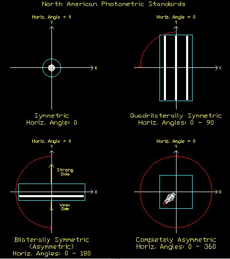
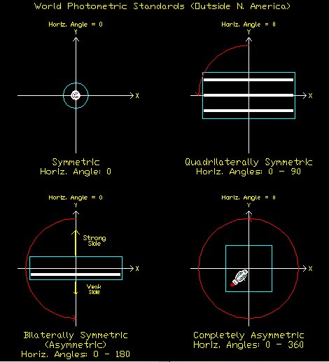
Distribution
As Photopia has come to be more widely used in the architectural lighting industry, an increasing number of Photopia generated photometric files are being distributed by lighting manufacturers to their customers. By photometric files, we are referring to IES files in North America and TM-14 or EULUMDAT in other regions of the world.
The original intent of Photopia was to allow manufacturers to develop new designs more quickly and more cost effectively by evaluating their design ideas on their computer instead of building and testing each and every design alternative. Once the predicted design performance met the desired criteria, a prototype was built and physically tested. If the physical test did not meet the design requirements, then modifications would be made until the requirements were met. In many cases, this involved troubleshooting the design to ensure it was built to specifications, so that it matched what was modeled in Photopia.
Photopia is no longer only used in the development of new standard products. It is also used to model the performance of custom luminaires where the time from concept to installation does not allow for the classic product development cycle. Additionally, it is being used to model some existing products for which photometric testing was never before required. In these cases and others, some manufactures will distribute photometric files generated by Photopia.
Whenever a photometric file generated by Photopia is distributed to a customer, the data should be as accurate as possible. The consequences of the photometric data not being accurate can be very costly if you are called out to fix an installed job. The distribution of inaccurate data also hurts Photopia's reputation and therefore its overall value. So it is in everyone's interest to ensure photometric data generated by Photopia is as accurate as possible.
While Photopia's accuracy has been confirmed by our own experience as well as that of our customers, the accuracy is dependent upon several critical factors, including but not limited to the following:
For more information about the factors that affect the accuracy, see Appendix C of the User's Guide.
Guidelines for Distributing Photometric Files:
If you do distribute IES files generated by Photopia, then please follow this advice:
Thank you for your attention to this issue.
The Photopia Product Support Team
Labs
While Photopia is excellent for simulating photometry, there are often times when you must use a physical lab. These may include:
There are many labs available for photometric testing. We would recommend the following labs:
Application Software
Lighting Application Software is typically used by lighting designers, electrical engineers, or architects to determine how many of what type of luminaire are required in a given space to achieve a certain light level or effect. There are currently several pieces of lighting application software that are widely used.
- AGi32 - Commercial software widely used by lighting designers.
- Visual - Software from Acuity Brands Lighting.
- Relux - Software sponsored by manufacturers, free for users.
- DIALux - Software sponsored by manufacturers, free for users.
* This list is not meant to be comprehensive or an endorsement of any particular software, but merely as a resource for our customers.
Tutorials
Analyze DWG Luminaire
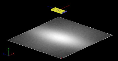
Skills Covered:
- Setting up Raytrace and Photometric Settings
- Viewing Output
Downloads:
- PDF Tutorial - Also located under Help / Beginner Tutorials in Photopia
Extruded Garage Lens
Skills Covered:
- Creating an Extruded Symmetric Prismatic Refractor
- Adjusting Aiming of Refractor
- Adding End Caps and Fillets
Downloads:
- PDF Tutorial - Also located under Help / Advanced Tutorials in Photopia
Fresnel Lens
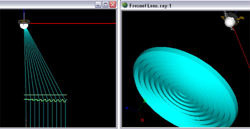
Skills Covered:
- Creating a Revolved Prismatic Refractor
- Switching from Prismatic to Smooth
- Switching Control from Inside to Outside
- Adding Peak and Valley Fillets
Downloads:
- PDF Tutorial - Also located under Help / Beginner Tutorials in Photopia
Import DWG Luminaire
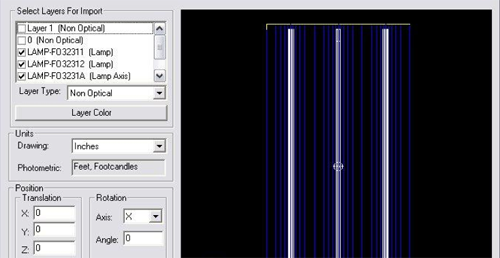
Skills Covered:
- Importing a DWG File using the Luminaire Import Wizard
- Assigning Material by Layer
Downloads:
- PDF Tutorial - Also located under Help / Beginner Tutorials in Photopia
LED Collimator
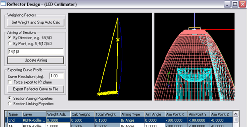
Skills Covered:
- Creating Revolved Refractor
- Linking Multiple Parametric Profiles
- Using Parametric Polylines with Arc Segments
Downloads:
- PDF Tutorial - Also located under Help / Advanced Tutorials in Photopia
LED Reflector
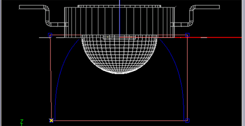
Skills Covered:
- Creating an Extruded Symmetric Reflector
- Specifying Anisotropic Material Orientation
Downloads:
- PDF Tutorial - Also located under Help / Advanced Tutorials in Photopia
Linear Fluorescent Highbay
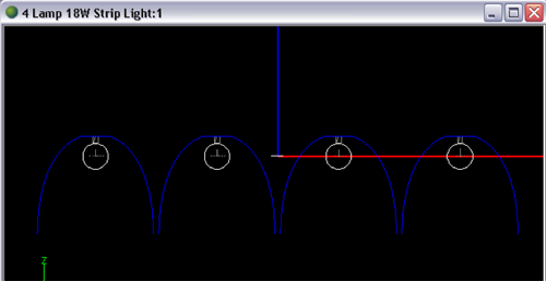
Skills Covered:
- Creating an Extruded Symmetric Reflector
- Arraying a Parametric Reflector and Lamps
Downloads:
- PDF Tutorial - Also located under Help / Advanced Tutorials in Photopia
Revolved Reflector
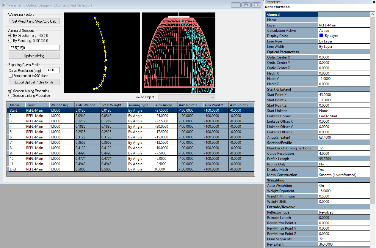
Skills Covered:
- Creating a Revolved Reflector
- Adjusting Aiming of Reflector
Downloads:
- PDF Tutorial - Also located under Help / Beginner Tutorials in Photopia
Roadway Reflector
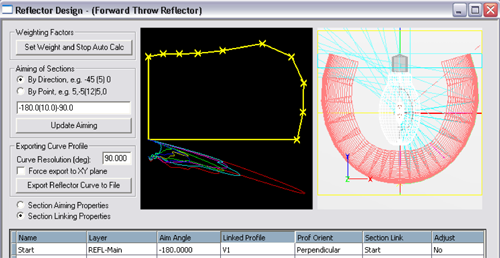
Skills Covered:
- Using Horizontal and Vertical Linked Profiles
- Advanced Raytrace Parameters
- Viewing Roadway Output
Downloads:
- PDF Tutorial - Also located under Help / Advanced Tutorials in Photopia
Skylight
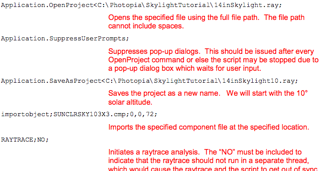
Skills Covered:
- Using scripting to build projects
- Using Batch Raytracing
- Using Sun and Sky Dome lamp models
Downloads:
- PDF Tutorial - Also located under Help / Advanced Tutorials in Photopia
Type V Lens
Skills Covered:
- Creating a Smooth Refractor
- Modifying Base Profile of Refractor
- Arraying a Refractor
Downloads:
- PDF Tutorial - Tutorial - Also Located under Help / Advanced Tutorials in Photopia
Type III Lens
Skills Covered:
- Creating a Smooth Refractor
- Modifying Base Profile of Refractor
- Lofting PODT profiles
Downloads:
Wall Wash Reflector
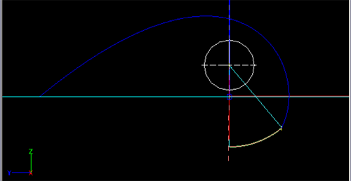
Skills Covered:
- Creating an Extruded Asymmetric Reflector
- Adjusting Aiming of Reflector
- Linking Multiple Reflectors
Downloads:
- PDF Tutorial - Also located under Help / Advanced Tutorials in Photopia
Compute Fluence for UVC Disinfection
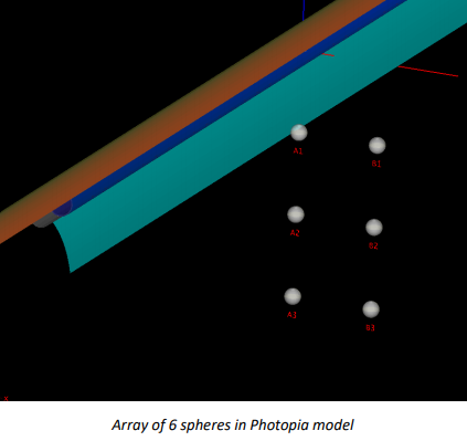
Skills Covered:
- Compute Fluence Rate
Downloads:
Analyze A Diffusion Lens
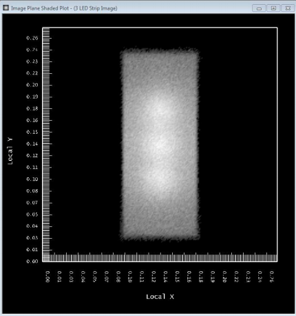
Skills Covered:
- Using an Imaging Lens
Downloads: