Contact Us
LTI Optics is always striving to improve customer support and provide you timely product updates and information to increase your productivity. If you have questions about your software, we invite you to review the sections below and check for new product downloads.
You may email support inquiries to us at the follow address: 
Should you need to call us, our support hours are 8 AM - 5 PM MST. Please review the technical support policy. Our technical support staff can be reached at 720-891-0030.
Policy
For
It is beyond the scope of standard technical support to create a full custom template or report for you. You can create a custom template yourself using the information on this page. It will be helpful if you have a knowledge of HTML and XML as these are the languages of the reports.
If you're not comfortable editing the HTML and XML configuration files to create a custom report, we are happy to offer this as a service. You'll just provide us with a template to match and we'll create all the custom files for your report. Email for a quote.
Install and Licensing
Install
Licensing
To license a standalone
Saving and Exporting
photopia | reports creates vector plots and html tables, which allow you to export web and print ready reports directly into your page layout software like Adobe InDesign.
Plots can be saved as SVG and PNG files.
Reports can be saved as PNG and HTML files.
Both Plots and Reports can be printed to PDF files.
Saving to PNG
When viewing a plot or report, choose the Save button and specify the file name for the PNG file. By default the export will be at the window resolution. To modify the resolution, before exporting, choose Settings > Image Resolution and set the pixel value for the smallest side of the image.
Saving to SVG
When viewing a plot, choose the Save button and specify the file name for the SVG file.
Saving to HTML
When viewing a plot or report, choose the Save button and specify the file name for the HTML file. By default the export will be at the window resolution. The HTML file was designed for the Microsoft Edge browser, so if it is opened in another browser it may not render the same.
Printing to PDF
Right click in the plot or report window and choose Print. You'll need to set the page margins and page scale to ensure that you fit the data onto the page.
In Windows 10 you can print directly to a PDF. In earlier versions you'll need a PDF print driver, like Adobe Acrobat, CutePDF, or the DiaLUX PDF printer.
Batch Export
The output from an entire set of IES or LDT files can be saved to the same format using command line parameters.
"C:\Program Files (x86)\LTI Optics\Reports\photopiareports.exe export input="C:\temp\*.ies" type=html configuration="C:\ProgramData\LTI Optics\Reports\CustomStyle\Our Custom HTML Template.xml" > temp.log
The export argument requires an input file or files and supports wildcards.
The type argument can be PNG | JPG | HTML | SVG | TXT.
The configuration argument specifies the configuration file, which must be compatible with the requested type.
The output file will have the same name as the IES or LDT file, with an extension based on the export type.
In order to save a batch of results to PDFs, you'll need to follow this process:
- Use Batch Export to create HTML files for each IES file.
- For each HTML file, you can use Chrome's headless printing option to create a PDF. Since you need to call each HTML explicitly to generate a corresponding PDF, you may need to program this in a batch file, VBA, Python or any other language you're familiar with. LTI Optics can offer this as a service as well.
"C:\Program Files (x86)\LTI Optics\Reports\photopiareports.exe export input="C:\temp\*.ies" type=html configuration="C:\ProgramData\LTI Optics\Reports\CustomStyle\OurCustomHTMLTemplate.xml" > temp.log
"C:\Program Files (x86)\Google\Chrome\Application\chrome.exe --headless --disable-gpu --print-to-pdf="C:\temp\MyNewPDFFile.pdf" "C:\temp\MyExistingHTMLFile.html"
Create a Custom Plot
You can customize any of the plots or data tables by creating a new style. The easiest way to do this is by copying an existing item that is similar and modifying it.
Location
All default style documents are stored here:
C:\Program Files (x86)\LTI Optics\Reports\Style\
The Program Files and Program Data folders may be hidden on your system. The easiest way to get there is by copying and pasting the paths above into the address bar of a Windows Explorer window.
In this folder, find a style that you want to create a modification of. For each style, there will be an .xml file that specifies the configuration and a .png file that is a preview of the plot used in the program interface. Copy both of these files.
Copy Files
Custom styles need to be placed in this location:
C:\ProgramData\LTI Optics\Reports\CustomStyle\
The Program Files and Program Data folders may be hidden on your system. The easiest way to get there is by copying and pasting the paths above into the address bar of a Windows Explorer window.
Paste the two files into the ProgramData folder and rename them with a new name. Note that the first part of the name IntensityPlot - must remain since it defines the particular plot or table type that the files apply to.
Thumbnail Icon
Each plot has a thumbnail icon. Creating a new thumbnail icon for your custom plot will make it easy to find in the program in the future. Custom icons need to be placed in this location:
C:\ProgramData\LTI Optics\Reports\CustomStyle\.
You can download the Gimp template file here to create your custom icon with. Open the file, edit text, layers and logos to create a logo you like, then export this as a .png file to the CustomStyle folder.
Modify Files
Open the xml file in a text editor and edit the values based on what you want to change. This page contains details of what most elements do.
You can manually create a preview image, or you can export an image from the tool and use that as the preview image.
Common Elements
Pixels, Points and Vectors
The Photometric Reports software generates all graphics as vector artwork, so they can be scaled to very high resolution.
Throughout the configuration, some items will be referenced as pixel values (either thickness or position) and fonts as point values. These are not actual pixels, but coordinates used to create the vectors. Some items are referenced as a percentage of the overall plot size.
Color Systems
Colors can be specified in the following formats:
- CIE_RGB: scaled 0-255
<type>CIE_RGB</type>
		<value>255,255,255</value>
- sRGB: scaled 0-255
<type>sRGB</type>
		<value>255,255,255</value>
- HSL: scaled 0-1
<type>HSL</type>
		<value>0.5,0.25,0.1</value>
- NULL_COLOR: can be used to turn off an element or make it fully transparent
<type>NULL_COLOR</type>
		<value>0,0,0</value>
Font Settings
Fonts are specified using the following block. Font family is similar to html/css referencing. Font size is specified in points.
<fontstyle>
			<family>Tahoma</family>
			<fillcolor>
				<type>HSL</type>
				<value>0.5,0.25,0.1</value>
			</fillcolor>
			<strokecolor>
				<type>HSL</type>
				<value>0.5,0.25,0.1</value>
			</strokecolor>
			<strokewidth>2</strokewidth>
			<fontsize>10</fontsize>
		</fontstyle>
Common Elements
Fill Color: sets the color of the fill, using any of the Color Systems above
<fillcolor>
			<type>HSL</type>
			<value>0.5,0.25,0.1</value>
		</fillcolor>
Opacity: sets the opacity of the fill, scaled 0-1
<opacity>0.5</opacity>
Stroke Color: sets the color of the stroke, using any of the Color Systems above
<strokecolor>
			<type>HSL</type>
			<value>0.5,0.25,0.1</value>
		</strokecolor>
Stroke Width: sets the width of the stroke in pixels
<strokewidth>3</strokewidth>
Hiding or Turning Off Items
Within plots, the best way to turn off or hide a particular item is to set the color of that item to NULL_COLOR.
<type>NULL_COLOR</type>
			<value>0,0,0</value>
IES Based Report
File Naming & Thumbnail Image
The file name must begin with the words "IESReport" and can be followed by any other text. A thumbnail image with a square aspect ratio should be placed alongside the xml file with the same name.
Example
An IES Report is a collection of plots and tables that is rendered as HTML. The file contains style directives as well as information for each plot and table.
<report>
			<style>
				body {
					font-family: "Century Gothic Bold";
				}

				#IntensityTable,
				#LuminaireLuminance {
					table-layout: auto;
				}
			</style>
			<fragment><![CDATA[<h1>Photometric Report</h1>]]></fragment>
			<HeaderTableConfiguration>
				<id>HeaderTable</id>
				<columnlabels></columnlabels>
				<includekeys>TESTLAB,MANUFAC</includekeys>
			</HeaderTableConfiguration>
			...
			other reports and plots
			...

		</report>
Style
The Style element is filled with CSS3 styles for formatting the report.
<style>
			body {
				font-family: "Century Gothic Bold";
			}

			#IntensityTable,
			#LuminaireLuminance {
				table-layout: auto;
			}
		</style>
Fragment
The fragment element is used for direct HTML entities that will be placed into the report. Use this element for any formatting or static text. Items within a fragment should be contained within a CData entity to preserve characters.
<fragment><![CDATA[<h1>Photometric Report</h1>]]></fragment>
CData
The CData element allows proper transfer of HTML from the report file to the final display.
<![CDATA[<h1>Photometric Report</h1>]]>
Candela/Intensity Polar Plots
File Naming & Thumbnail Image
The file name must begin with the words "IntensityPlot" and can be followed by any other text. A thumbnail image with a square aspect ratio should be placed alongside the xml file with the same name.
View Size
The size, in pixels, of the view.
<viewdimensions>1000,1000<viewdimensions/>
Interpolation
Controls the interpolation of the plotted candela data between values in the data file.
- 0 = No interpolation
- 1 = Linear
- 2 = Hermite (default)
- 3 = Cosine
- 4 = Catmull Rom
<interpolation>2<interpolation/>
View Style
Controls the overall window background and border.
<viewstyle>
			<fillcolor>
				<type>sRGB</type>
				<value>255,255,255</value>
			</fillcolor>
			<strokecolor>
				<type>sRGB</type>
				<value>128,128,128</value>
			</strokecolor>
			<strokewidth>0</strokewidth>
			<opacity>0</opacity>
		</viewstyle>
Border Style
Controls the plot background and border.
<borderstyle>
			<fillcolor>
				<type>sRGB</type>
				<value>255,255,255</value>
			</fillcolor>
			<strokecolor>
				<type>sRGB</type>
				<value>128,128,128</value>
			</strokecolor>
			<strokewidth>0</strokewidth>
			<opacity>0</opacity>
		</borderstyle>
Legend
Controls the plot background and border.
The legend position can be left,right,top, or bottom.
The legend offset is a value in percent of the view extents that the legend is offset from the base position.
The columnwidths are in percent of the view extents. The first number is the angle text, the second is the line illustration.
<showlegend>true</showlegend>
		<legend>
			<position>right</position>
			<offset>0,-0.3</offset>
			<columnwidths>0.08,0.04</columnwidths>
			<borderstyle>
				<fillcolor>
					<type>NULL_COLOR</type>
					<value>0,0,0</value>
				</fillcolor>
				<strokecolor>
					<type>SRGB</type>
					<value>0,0,0</value>
				</strokecolor>
				<strokewidth>1</strokewidth>
				<opacity>1</opacity>
			</borderstyle>
			<fontstyle>
				<family>Tahoma</family>
				<fillcolor>
					<type>CIE_RGB</type>
					<value>0,0,0</value>
				</fillcolor>
				<strokecolor>
					<type>CIE_RGB</type>
					<value>0,0,0</value>
				</strokecolor>
				<strokewidth>0</strokewidth>
				<fontsize>10</fontsize>
			</fontstyle>
		</legend>
Half Plane
When set to true, all data is displayed on the right half of the plot. When set to false, the data is plotted on the left and right half in full plane pairs.
<halfplane>true<halfplane/>
Uplight
When set to true, uplight and downlight data is plotted. When set to false, only downlight data is plotted.
<uplight>true<uplight/>
Zoom To Data
When set to 0.0, the plots boundaries will be circular. When set to anything from 0.0 to 1.0, the plot will be zoomed to fit the data. At 1.0 the plot exactly fits the data, at 0.9, there is a 10% padding.
<zoomtofit>0.0<zoomtofit/>
Data Style Gradient
The style gradient specifies the start and end horizontal angle styles and then creates a gradient between this.
<seriesstylegradient>
			<dataseriesstyle>
				<fillcolor>
					<type>HSL</type>
					<value>0,1,0.5</value>
				</fillcolor>
				<strokecolor>
					<type>HSL</type>
					<value>0,1,0.5</value>
				</strokecolor>
				<strokewidth>2</strokewidth>
				<opacity>0</opacity>
			</dataseriesstyle>
			<dataseriesstyle>
				<fillcolor>
					<type>HSL</type>
					<value>0.83,1,0.5</value>
				</fillcolor>
				<strokecolor>
					<type>HSL</type>
					<value>0.83,1,0.5</value>
				</strokecolor>
				<strokewidth>2</strokewidth>
				<opacity>0</opacity>
			</dataseriesstyle>
		</seriesstylegradient>
Data Style Override
The series style override allows you to explicitly set the style for individual horizontal planes of data. This element is not necessary. The <key> is the horizontal plane in degrees.
Secondary card title
Some quick example text to build on the card title and make up the bulk of the card's content.
<seriesstyleoverride>
			<dataseriesstyle>
				<key>0</key>
				<value>
					<fillcolor>
						<type>SRGB</type>
						<value>255,230,0</value>
					</fillcolor>
					<strokecolor>
						<type>sRGB</type>
						<value>255,204,0</value>
					</strokecolor>
					<strokewidth>2</strokewidth>
					<opacity>.5</opacity>
				</value>
			</dataseriesstyle>
		</seriesstyleoverride>
Title
The plot title text and style.
<title>Polar Plot</title>
		<titlefont>
			<family>Tahoma</family>
			<fillcolor>
				<type>HSL</type>
				<value>0,0,0</value>
			</fillcolor>
			<strokecolor>
				<type>NULL_COLOR</type>
				<value>0,0,0</value>
			</strokecolor>
			<strokewidth>1</strokewidth>
			<fontsize>20</fontsize>
		</titlefont>
Radius Markers
The radius markers are the circles at certain candela values.
<radiusmarkerstart>0.0</radiusmarkerstart>
		<radiusmarkerincrement>0.0</radiusmarkerincrement>
		<radiusmarkermajordivisor>1</radiusmarkermajordivisor>
		<radiusmarkerminordivisor>1</radiusmarkerminordivisor>
		<radiusminorfontstyle>
			<family>Tahoma</family>
			<fillcolor>
				<type>HSL</type>
				<value>0,0,0.8</value>
			</fillcolor>
			<strokecolor>
				<type>HSL</type>
				<value>0,0,0.8</value>
			</strokecolor>
			<strokewidth>0</strokewidth>
			<fontsize>12</fontsize>
		</radiusminorfontstyle>
		<radiusminorlinestyle>
			<fillcolor>
				<type>NULL_COLOR</type>
				<value>0,0,0</value>
			</fillcolor>
			<strokecolor>
				<type>HSL</type>
				<value>0,0,0.8</value>
			</strokecolor>
			<strokewidth>0.5</strokewidth>
			<opacity>1</opacity>
		</radiusminorlinestyle>
		<radiusmajorfontstyle>
			<family>Tahoma</family>
			<fillcolor>
				<type>HSL</type>
				<value>0,0,0.8</value>
			</fillcolor>
			<strokecolor>
				<type>HSL</type>
				<value>0,0,0.8</value>
			</strokecolor>
			<strokewidth>0</strokewidth>
			<fontsize>12</fontsize>
		</radiusmajorfontstyle>
		<radiusmajorlinestyle>
			<fillcolor>
				<type>NULL_COLOR</type>
				<value>0,0,0</value>
			</fillcolor>
			<strokecolor>
				<type>HSL</type>
				<value>0,0,.5</value>
			</strokecolor>
			<strokewidth>0.7</strokewidth>
			<opacity>1</opacity>
		</radiusmajorlinestyle>
Angle Markers
The angle markers are the lines from the center of the plot for each vertical angle.
<anglemarkerincrement>0.174533</anglemarkerincrement>
		<anglemarkermajordivisor>1</anglemarkermajordivisor>
		<anglemarkerminordivisor>1</anglemarkerminordivisor>
		<angleminorfontstyle>
			<family>Tahoma</family>
			<fillcolor>
				<type>HSL</type>
				<value>0,0,0.5</value>
			</fillcolor>
			<strokecolor>
				<type>HSL</type>
				<value>0,0,0.5</value>
			</strokecolor>
			<strokewidth>0</strokewidth>
			<fontsize>12</fontsize>
		</angleminorfontstyle>
		<angleminorlinestyle>
			<fillcolor>
				<type>NULL_COLOR</type>
				<value>0,0,0</value>
			</fillcolor>
			<strokecolor>
				<type>HSL</type>
				<value>0,0,0.5</value>
			</strokecolor>
			<strokewidth>0.5</strokewidth>
			<opacity>1</opacity>
		</angleminorlinestyle>
		<anglemajorfontstyle>
			<family>Tahoma</family>
			<fillcolor>
				<type>HSL</type>
				<value>0,0,0.7</value>
			</fillcolor>
			<strokecolor>
				<type>HSL</type>
				<value>0,0,0.7</value>
			</strokecolor>
			<strokewidth>0</strokewidth>
			<fontsize>12</fontsize>
		</anglemajorfontstyle>
		<anglemajorlinestyle>
			<fillcolor>
				<type>NULL_COLOR</type>
				<value>0,0,0</value>
			</fillcolor>
			<strokecolor>
				<type>HSL</type>
				<value>0,0,0.7</value>
			</strokecolor>
			<strokewidth>0.7</strokewidth>
			<opacity>1</opacity>
		</anglemajorlinestyle>
Candela/Intensity XY Plots
File Naming & Thumbnail Image
The file name must begin with the words "IntensityXYPlot" and can be followed by any other text. A thumbnail image with a square aspect ratio should be placed alongside the xml file with the same name.
Within a report the main keyword is:
<IntensityXYPlotConfiguration>
Interpolation
Controls the interpolation of the plotted candela data between values in the data file.
- 0 = No interpolation
- 1 = Linear
- 2 = Hermite (default)
- 3 = Cosine
- 4 = Catmull Rom
<interpolation>2<interpolation/>
View Dimensions
The size, in pixels, of the view.
<viewdimensions>500,500<viewdimensions/>
Padding
The padding around the plot inside the View Dimensions, in %.
<padding>0.04,0.04<padding/>
Plot Dimensions
The % size of the View Dimensions that the plot occupies.
<plotdimensions>.7,.8<plotdimensions/>
Plot Position
The % offset inside the View Dimension from the lower left hand corner.
<plotposition>.1,.07<plotposition/>
View Style
Controls the overall window background and border.
<viewstyle>
			<fillcolor>
				<type>sRGB</type>
				<value>255,255,255</value>
			</fillcolor>
			<strokecolor>
				<type>sRGB</type>
				<value>128,128,128</value>
			</strokecolor>
			<strokewidth>0</strokewidth>
			<opacity>0</opacity>
		</viewstyle>
Border Style
Controls the plot background and border.
<borderstyle>
			<fillcolor>
				<type>sRGB</type>
				<value>255,255,255</value>
			</fillcolor>
			<strokecolor>
				<type>sRGB</type>
				<value>128,128,128</value>
			</strokecolor>
			<strokewidth>0</strokewidth>
			<opacity>0</opacity>
		</borderstyle>
Legend
Controls the plot background and border.
The legend position can be left,right,top, or bottom.
The legend offset is a value in percent of the view extents that the legend is offset from the base position.
The columnwidths are in percent of the view extents. The first number is the angle text, the second is the line illustration.
<showlegend>true</showlegend>
		<legend>
			<position>right</position>
			<offset>0,-0.3</offset>
			<columnwidths>0.08,0.04</columnwidths>
			<borderstyle>
				<fillcolor>
					<type>NULL_COLOR</type>
					<value>0,0,0</value>
				</fillcolor>
				<strokecolor>
					<type>SRGB</type>
					<value>0,0,0</value>
				</strokecolor>
				<strokewidth>1</strokewidth>
				<opacity>1</opacity>
			</borderstyle>
			<fontstyle>
				<family>Tahoma</family>
				<fillcolor>
					<type>CIE_RGB</type>
					<value>0,0,0</value>
				</fillcolor>
				<strokecolor>
					<type>CIE_RGB</type>
					<value>0,0,0</value>
				</strokecolor>
				<strokewidth>0</strokewidth>
				<fontsize>10</fontsize>
			</fontstyle>
		</legend>
Data Style Gradient
The style gradient specifies the start and end horizontal angle styles and then creates a gradient between this.
<seriesstylegradient>
			<dataseriesstyle>
				<fillcolor>
					<type>HSL</type>
					<value>0,1,0.5</value>
				</fillcolor>
				<strokecolor>
					<type>HSL</type>
					<value>0,1,0.5</value>
				</strokecolor>
				<strokewidth>2</strokewidth>
				<opacity>0</opacity>
			</dataseriesstyle>
			<dataseriesstyle>
				<fillcolor>
					<type>HSL</type>
					<value>0.83,1,0.5</value>
				</fillcolor>
				<strokecolor>
					<type>HSL</type>
					<value>0.83,1,0.5</value>
				</strokecolor>
				<strokewidth>2</strokewidth>
				<opacity>0</opacity>
			</dataseriesstyle>
		</seriesstylegradient>
Data Style Override
The series style override allows you to explicitly set the style for individual horizontal planes of data. This element is not necessary. The <key> is the horizontal plane in degrees.
<seriesstyleoverride>
			<dataseriesstyle>
				<key>0</key>
				<value>
					<fillcolor>
						<type>SRGB</type>
						<value>255,230,0</value>
					</fillcolor>
					<strokecolor>
						<type>sRGB</type>
						<value>255,204,0</value>
					</strokecolor>
					<strokewidth>2</strokewidth>
					<opacity>.5</opacity>
				</value>
			</dataseriesstyle>
		</seriesstyleoverride>
Title
The plot title text and style.
<title>X-Y Intensity Plot</title>
		<titlefont>
			<family>Tahoma</family>
			<fillcolor>
				<type>HSL</type>
				<value>0,0,0</value>
			</fillcolor>
			<strokecolor>
				<type>NULL_COLOR</type>
				<value>0,0,0</value>
			</strokecolor>
			<strokewidth>1</strokewidth>
			<fontsize>20</fontsize>
		</titlefont>
Axis Markers
The axis markers for the x and y axis. The x and y axis can have unique intervals, but share formatting.
<xmarkerstart>0.0</xmarkerstart>
		<xmarkerincrement>0.0</xmarkerincrement>
		<xmarkermajordivisor>1</xmarkermajordivisor>
		<xmarkerminordivisor>1</xmarkerminordivisor>
		<ymarkerstart>0.0</ymarkerstart>
		<ymarkerincrement>0.0</ymarkerincrement>
		<ymarkermajordivisor>1</ymarkermajordivisor>
		<ymarkerminordivisor>1</ymarkerminordivisor>

		<minorMarkerFontStyle>
			<family>Tahoma</family>
			<fillcolor>
				<type>HSL</type>
				<value>0,0,0.8</value>
			</fillcolor>
			<strokecolor>
				<type>HSL</type>
				<value>0,0,0.8</value>
			</strokecolor>
			<strokewidth>0</strokewidth>
			<fontsize>12</fontsize>
		</minorMarkerFontStyle>
		<minorMarkerLineStyle>
			<fillcolor>
				<type>NULL_COLOR</type>
				<value>0,0,0</value>
			</fillcolor>
			<strokecolor>
				<type>HSL</type>
				<value>0,0,0.8</value>
			</strokecolor>
			<strokewidth>0.5</strokewidth>
			<opacity>1</opacity>
		</minorMarkerLineStyle>

		<majorMarkerFontStyle>
			<family>Tahoma</family>
			<fillcolor>
				<type>HSL</type>
				<value>0,0,0.8</value>
			</fillcolor>
			<strokecolor>
				<type>HSL</type>
				<value>0,0,0.8</value>
			</strokecolor>
			<strokewidth>0</strokewidth>
			<fontsize>12</fontsize>
		</majorMarkerFontStyle>
		<majorMarkerLineStyle>
			<fillcolor>
				<type>NULL_COLOR</type>
				<value>0,0,0</value>
			</fillcolor>
			<strokecolor>
				<type>HSL</type>
				<value>0,0,0.8</value>
			</strokecolor>
			<strokewidth>0.5</strokewidth>
			<opacity>1</opacity>
		</majorMarkerLineStyle>
Iso-Illuminance Plots
File Naming & Thumbnail Image
The file name must begin with the words "ISOIlluminance" and can be followed by any other text. A thumbnail image with a square aspect ratio should be placed alongside the xml file with the same name.
Within a report the main keyword is:
<FluxDensityIntensityContourReport>
Roadway Annotations
Controls the display of the peak intensity and 50% intensity labels common on roadway plots.
- 0 = No roadway annotations
- 1 = Includes roadway annotations
<roadwayannotations>0</roadwayannotations>
XY MHs or Distance
Sets the X and Y axis to be defined in units of mounting height or absolute distance.
- 0 = Plot is in multiples of mounting height
- 1 = Plot is in absolute distances
<domain-range-in-mounting-heights>0</domain-range-in-mounting-heights>
XY Plot Extents
Specifies the extents of the plot in x and y dimensions (values are either mounting heights or absolute based on the <domain-range-in-mounting-heights> element) with the following convention:
left x, right x, lower y, upper y
<domain-range>0,20,-5,5</domain-range>
Mounting Height
Sets the mounting height of the luminaire, either in feet to display footcandles or meters to display lux.
<mounting-height>10</mounting-height>
Mounting Orientation
Allows you to adjust the aiming of the luminaire using the standard Orientation, Tilt, and Spin values defined by the IES.
<mountingorientation>270, 60, 0</mountingorientation>
Labels
Sets the text value of various labels. Leave an element empty to omit a label.
<housesidelabel>House Side</housesidelabel>
		<streetsidelabel>Street Side</streetsidelabel>
		<halfmaxcandelatracelabel>Half Max Candela Trace: </halfmaxcandelatracelabel>
		<maxcandelapointlabel>Max Candela Point: </maxcandelapointlabel>
		<shortlabel>Short</shortlabel>
		<mediumlabel>Medium</mediumlabel>
		<longlabel>Long</longlabel>
		<typeilabel>Type I</typeilabel>
		<typeiilabel>Type II</typeiilabel>
		<typeiiilabel>Type III</typeiiilabel>
		<typeivlabel>Type IV</typeivlabel>
		<typevlabel>Type V</typevlabel>
		<mountingheightunitlabel>ft</mountingheightunitlabel>
		<mountingheightlabel>Mounting Height: </mountingheightlabel>

		<leftaxislabel>Y Distance [ft]</leftaxislabel>
		<bottomaxislabel>X Distance [ft]</bottomaxislabel>
		<titlelabel>Iso-Illuminance</titlelabel>

		<contourfluxunitlabel>fc</contourfluxunitlabel>
		<contourintensityunitlabel>cd</contourintensityunitlabel>
		<legendunitlabel>fc</legendunitlabel>
Font Styles
Using the common font setting, you can set the font of each label type independently.
<TitleFontStyle>
			<family>Tahoma</family>
			<fillcolor>
				<type>HSL</type>
				<value>0,0,0.8</value>
			</fillcolor>
			<strokecolor>
				<type>HSL</type>
				<value>0,0,0.8</value>
			</strokecolor>
			<strokewidth>0</strokewidth>
			<fontsize>12</fontsize>
		</TitleFontStyle>

		<axisfontstyle>...</axisfontstyle>
		<leftaxisfontstyle>...</leftaxisfontstyle>
		<rangelabelsfontstyle>...</rangelabelsfontstyle>
		<countourlabelsfontstyle>...</contourlabelsfontstyle>
		<roadwaylabelsfontstyle>...</roadwaylabelsfontstyle>
		<legendfontstyle>...</legendfontstyle>
		<legendplanedatafontstyle>...</legendplanedatafontstyle>
		<scalelabelsfontstyle>...</scalelabelsfontstyle>
Iso-Illuminance Contours
Iso-Illuminance Contours
Contours can be specified at specific illuminance values using the <contours> element.
<contours>1,2,6,20</contours>
Contours can be specified at specific percents of the peak illuminance value using the <percent-contours> element with multiple values.
<percent-contours>0.05,0.1,0.5,0.99</percent-contours>
Contours can be specified at uniform percent increments of the peak illuminance values using the <percent-contours> element with a single value, such as every 5% in the example below.
<contours>0.05</contours>
Contours labels can be set to on (1) or off (0).
<contourlabel>1</contourlabel>
Contours labels can be rounded to a specified number of decimal places.
<contourlabelsdecimalrounding>0.01</contourlabelsdecimalrounding>
Contour style can be specified as fixed for all contours.
<contourstyle>stroke:white; fill:none; stroke-width: 0.2px</contourstyle>
Or contour style can be specified as a gradient.
<contourstylegradient>
			<start>
				<fillcolor>
					<type>HSL</type>
					<value>0.8, 1.0, 0.5</value>
				</fillcolor>
				<strokecolor>
					<type>HSL</type>
					<value>0.8, 1.0, 0.5</value>
				</strokecolor>
				<strokewidth>0</strokewidth>
				<opacity>0</opacity>
			</start>
			<end>
				<fillcolor>
					<type>HSL</type>
					<value>0.0, 1.0, 0.5</value>
				</fillcolor>
				<strokecolor>
					<type>HSL</type>
					<value>0.0, 1.0, 0.5</value>
				</strokecolor>
				<strokewidth>0</strokewidth>
				<opacity>0</opacity>
			</end>
		<contourstylegradient>
Shaded Illuminance
The plane background is filled with a gradient where the start and end values are specified and apply to the max and minimum values on the plane. This is essentially a false color illuminance plot.
<planedatastylegradient>
			<start>
				<fillcolor>
					<type>HSL</type>
					<value>0.8, 1.0, 0.5</value>
				</fillcolor>
				<strokecolor>
					<type>HSL</type>
					<value>0.8, 1.0, 0.5</value>
				</strokecolor>
				<strokewidth>0</strokewidth>
				<opacity>0</opacity>
			</start>
			<end>
				<fillcolor>
					<type>HSL</type>
					<value>0.0, 1.0, 0.5</value>
				</fillcolor>
				<strokecolor>
					<type>HSL</type>
					<value>0.0, 1.0, 0.5</value>
				</strokecolor>
				<strokewidth>0</strokewidth>
				<opacity>0</opacity>
			</end>
		<planedatastylegradient>
A legend will be displayed on the right side of the plot.
<planedatalegendwidht>10</planedatalegendwidth>
		<legendplanedatafontstyle>...</legendplanedatafontstyle>
Plane Data Resolution sets the number of points in X and Y on the plot that will be used to compute the illuminance values.
<planedataresolution>120</planedataresolution>
Plane Data Unit allows the plane to display either illuminance (fluxdensity) or intensity.
<planedataunit>fluxdensity</planedataunit>
Grids
Independent major and minor grids can be setup on the plot. Major grids can be labeled, minor grids are just grid lines. Frequency is how often the grid should occur, and will match the units of the domain. Line styles can be specified as CSS styles.
<grid-horizontalaxis-major>
			<frequency>10</frequency>
			<line-display>true</line-display>
			<label-display>true</label-display>
			<line-style>stroke:white; fill:none; stroke-width: 0.2px</line-style>

			<line-style>true</line-style>
			<FontStyle>
				<family>Tahoma</family>
				<fillcolor>
					<type>HSL</type>
					<value>0,0,0.8</value>
				</fillcolor>
				<strokecolor>
					<type>HSL</type>
					<value>0,0,0.8</value>
				</strokecolor>
				<strokewidth>0</strokewidth>
				<fontsize>12</fontsize>
			</FontStyle>
		</grid-horizontalaxis-major>


		<grid-verticalaxis-major>...</grid-verticalaxis-major>


		<grid-horizontalaxis-minor>
			<frequency>10</frequency>
			<line-display>true</line-display>
			<line-style>stroke:white; fill:none; stroke-width: 0.2px</line-style>
		</grid-horizontalaxis-minor>


		<grid-verticalaxis-minor>...</grid-verticalaxis-minor>
View Dimensions
The size, in pixels, of the view.
<viewdimensions>500,500</viewdimensions>
Roadway CU XY Plots
File Naming & Thumbnail Image
The file name must begin with the words "CUXYPlot" and can be followed by any other text. A thumbnail image with a square aspect ratio should be placed alongside the xml file with the same name.
Within a report the main keyword is:
<CUXYPlotConfiguration>
Interpolation
Controls the interpolation of the plotted CU data between values in the data file.
- 0 = No interpolation
- 1 = Linear
- 2 = Hermite (default)
- 3 = Cosine
- 4 = Catmull Rom
<interpolation>2<interpolation/>
View Dimensions
The size, in pixels, of the view.
<viewdimensions>500,500<viewdimensions/>
Padding
The padding around the plot inside the View Dimensions, in %.
<padding>0.04,0.04<padding/>
Plot Dimensions
The % size of the View Dimensions that the plot occupies.
<plotdimensions>.7,.8<plotdimensions/>
Plot Position
The % offset inside the View Dimension from the lower left hand corner.
<plotposition>.1,.07<plotposition/>
View Style
Controls the overall window background and border.
<viewstyle>
			<fillcolor>
				<type>sRGB</type>
				<value>255,255,255</value>
			</fillcolor>
			<strokecolor>
				<type>sRGB</type>
				<value>128,128,128</value>
			</strokecolor>
			<strokewidth>0</strokewidth>
			<opacity>0</opacity>
		</viewstyle>
Border Style
Controls the plot background and border.
<borderstyle>
			<fillcolor>
				<type>sRGB</type>
				<value>255,255,255</value>
			</fillcolor>
			<strokecolor>
				<type>sRGB</type>
				<value>128,128,128</value>
			</strokecolor>
			<strokewidth>0</strokewidth>
			<opacity>0</opacity>
		</borderstyle>
Legend
Controls the plot background and border.
The legend position can be left,right,top, or bottom.
The legend offset is a value in percent of the view extents that the legend is offset from the base position.
The columnwidths are in percent of the view extents. The first number is the angle text, the second is the line illustration.
<showlegend>true</showlegend>
		<legend>
			<position>right</position>
			<offset>0,-0.3</offset>
			<columnwidths>0.08,0.04</columnwidths>
			<borderstyle>
				<fillcolor>
					<type>NULL_COLOR</type>
					<value>0,0,0</value>
				</fillcolor>
				<strokecolor>
					<type>SRGB</type>
					<value>0,0,0</value>
				</strokecolor>
				<strokewidth>1</strokewidth>
				<opacity>1</opacity>
			</borderstyle>
			<fontstyle>
				<family>Tahoma</family>
				<fillcolor>
					<type>CIE_RGB</type>
					<value>0,0,0</value>
				</fillcolor>
				<strokecolor>
					<type>CIE_RGB</type>
					<value>0,0,0</value>
				</strokecolor>
				<strokewidth>0</strokewidth>
				<fontsize>10</fontsize>
			</fontstyle>
		</legend>
Street Side Style
Specifies the style of the street side data line.
<streetSideStyle>
				<fillcolor>
					<type>HSL</type>
					<value>0,1,0.5</value>
				</fillcolor>
				<strokecolor>
					<type>HSL</type>
					<value>0,1,0.5</value>
				</strokecolor>
				<strokewidth>2</strokewidth>
				<opacity>0</opacity>
			</streetSideStyle>
		<streetSideLabel>Street side</streetSideLabel>
House Side Style
Specifies the house side style
<houseSideStyle>
				<fillcolor>
					<type>HSL</type>
					<value>0,1,0.5</value>
				</fillcolor>
				<strokecolor>
					<type>HSL</type>
					<value>0,1,0.5</value>
				</strokecolor>
				<strokewidth>2</strokewidth>
				<opacity>0</opacity>
			</houseSideStyle>
		<houseSideLabel>House side</houseSideLabel>
Mounting Heights
Specifies the spacing to mounting height ratios to compute and plot.
<mountingheights>0,1,2,3,4,5,6,7,8,9,10</mountingheights>
Title
The plot title text and style.
<title>Roadway CU Plot</title>
		<titlefont>
			<family>Tahoma</family>
			<fillcolor>
				<type>HSL</type>
				<value>0,0,0</value>
			</fillcolor>
			<strokecolor>
				<type>NULL_COLOR</type>
				<value>0,0,0</value>
			</strokecolor>
			<strokewidth>1</strokewidth>
			<fontsize>20</fontsize>
		</titlefont>
X Axis Labels
The style for the x axis.
<xaxisposition>0.0</xaxisposition>
		<xaxisstyle>
			<fillcolor>
				<type>HSL</type>
				<value>0,0,0</value>
			</fillcolor>
			<strokecolor>
				<type>NULL_COLOR</type>
				<value>0,0,0</value>
			</strokecolor>
			<strokewidth>1</strokewidth>
			<opacity>0</opacity>
		</xaxisstyle>
		<xaxislabel>Street width / Mounting height</xaxislabel>
		<xaxislabeloffset>0.05</xaxislabeloffset>
		<xaxislabelfont>
			<family>Tahoma</family>
			<fillcolor>
				<type>HSL</type>
				<value>0,0,0</value>
			</fillcolor>
			<strokecolor>
				<type>NULL_COLOR</type>
				<value>0,0,0</value>
			</strokecolor>
			<strokewidth>1</strokewidth>
			<fontsize>20</fontsize>
		</xaxislabelfont>
Y Axis Labels
The style for the y axis.
<yaxisposition>0.0</yaxisposition>
		<yaxisstyle>
			<fillcolor>
				<type>HSL</type>
				<value>0,0,0</value>
			</fillcolor>
			<strokecolor>
				<type>NULL_COLOR</type>
				<value>0,0,0</value>
			</strokecolor>
			<strokewidth>1</strokewidth>
			<opacity>0</opacity>
		</yaxisstyle>
		<yaxislabel>Coefficient of Utilization</yaxislabel>
		<yaxislabeloffset>0.05</yaxislabeloffset>
		<yaxislabelfont>
			<family>Tahoma</family>
			<fillcolor>
				<type>HSL</type>
				<value>0,0,0</value>
			</fillcolor>
			<strokecolor>
				<type>NULL_COLOR</type>
				<value>0,0,0</value>
			</strokecolor>
			<strokewidth>1</strokewidth>
			<fontsize>20</fontsize>
		</yaxislabelfont>
Axis Markers
The axis markers for the x and y axis. The x and y axis can have unique intervals, but share formatting.
<xmarkerstart>0.0</xmarkerstart>
		<xmarkerincrement>0.0</xmarkerincrement>
		<xmarkermajordivisor>1</xmarkermajordivisor>
		<xmarkerminordivisor>1</xmarkerminordivisor>
		<ymarkerstart>0.0</ymarkerstart>
		<ymarkerincrement>0.0</ymarkerincrement>
		<ymarkermajordivisor>1</ymarkermajordivisor>
		<ymarkerminordivisor>1</ymarkerminordivisor>

		<minorMarkerFontStyle>
			<family>Tahoma</family>
			<fillcolor>
				<type>HSL</type>
				<value>0,0,0.8</value>
			</fillcolor>
			<strokecolor>
				<type>HSL</type>
				<value>0,0,0.8</value>
			</strokecolor>
			<strokewidth>0</strokewidth>
			<fontsize>12</fontsize>
		</minorMarkerFontStyle>
		<minorMarkerLineStyle>
			<fillcolor>
				<type>NULL_COLOR</type>
				<value>0,0,0</value>
			</fillcolor>
			<strokecolor>
				<type>HSL</type>
				<value>0,0,0.8</value>
			</strokecolor>
			<strokewidth>0.5</strokewidth>
			<opacity>1</opacity>
		</minorMarkerLineStyle>

		<majorMarkerFontStyle>
			<family>Tahoma</family>
			<fillcolor>
				<type>HSL</type>
				<value>0,0,0.8</value>
			</fillcolor>
			<strokecolor>
				<type>HSL</type>
				<value>0,0,0.8</value>
			</strokecolor>
			<strokewidth>0</strokewidth>
			<fontsize>12</fontsize>
		</majorMarkerFontStyle>
		<majorMarkerLineStyle>
			<fillcolor>
				<type>NULL_COLOR</type>
				<value>0,0,0</value>
			</fillcolor>
			<strokecolor>
				<type>HSL</type>
				<value>0,0,0.8</value>
			</strokecolor>
			<strokewidth>0.5</strokewidth>
			<opacity>1</opacity>
		</majorMarkerLineStyle>
LCS Plots
File Naming & Thumbnail Image
The file name must begin with the words "LCSPlot" and can be followed by any other text. A thumbnail image with a square aspect ratio should be placed alongside the xml file with the same name.
Within a report the main keyword is:
<CUPlotConfiguration>
View Dimensions
The size, in pixels, of the view.
<viewdimensions>1000,1000</viewdimensions/>
Padding
The size padding around the plot, in a fraction.
<padding>.08,.08</padding/>
Value Type
0 to plot lumens(energy), 1 for % of lamp, 2 for % of luminaire.
<valuetype>0</valuetype/>
Series Style
Specifies for each zone the fill and stroke. The valid zones are BVH, BH, BM, VL, FVH, FH, FM, FL, UH and UL.
<seriesStyles>
			<BH>
				<fillcolor>
					<type>sRGB</type>
					<value>255,255,255</value>
				</fillcolor>
				<strokecolor>
					<type>sRGB</type>
					<value>128,128,128</value>
				</strokecolor>
				<strokewidth>0</strokewidth>
				<opacity>0</opacity>
			</BH>
			<BL>
				<fillcolor>
					<type>sRGB</type>
					<value>255,255,255</value>
				</fillcolor>
				<strokecolor>
					<type>sRGB</type>
					<value>128,128,128</value>
				</strokecolor>
				<strokewidth>0</strokewidth>
				<opacity>0</opacity>
			</BL>
		</seriesStyles>
Title
The plot title text and style.
<title>Polar Plot</title>
		<titlefont>
			<family>Tahoma</family>
			<fillcolor>
				<type>HSL</type>
				<value>0,0,0</value>
			</fillcolor>
			<strokecolor>
				<type>NULL_COLOR</type>
				<value>0,0,0</value>
			</strokecolor>
			<strokewidth>1</strokewidth>
			<fontsize>20</fontsize>
		</titlefont>
Radius Markers
The radius markers are the circles at certain candela values.
<radiusmarkerstart>0.0</radiusmarkerstart>
		<radiusmarkerincrement>0.0</radiusmarkerincrement>
		<radiusmarkermajordivisor>1</radiusmarkermajordivisor>
		<radiusmarkerminordivisor>1</radiusmarkerminordivisor>
		<radiusminorfontstyle>
			<family>Tahoma</family>
			<fillcolor>
				<type>HSL</type>
				<value>0,0,0.8</value>
			</fillcolor>
			<strokecolor>
				<type>HSL</type>
				<value>0,0,0.8</value>
			</strokecolor>
			<strokewidth>0</strokewidth>
			<fontsize>12</fontsize>
		</radiusminorfontstyle>
		<radiusminorlinestyle>
			<fillcolor>
				<type>NULL_COLOR</type>
				<value>0,0,0</value>
			</fillcolor>
			<strokecolor>
				<type>HSL</type>
				<value>0,0,0.8</value>
			</strokecolor>
			<strokewidth>0.5</strokewidth>
			<opacity>1</opacity>
		</radiusminorlinestyle>
		<radiusmajorfontstyle>
			<family>Tahoma</family>
			<fillcolor>
				<type>HSL</type>
				<value>0,0,0.8</value>
			</fillcolor>
			<strokecolor>
				<type>HSL</type>
				<value>0,0,0.8</value>
			</strokecolor>
			<strokewidth>0</strokewidth>
			<fontsize>12</fontsize>
		</radiusmajorfontstyle>
		<radiusmajorlinestyle>
			<fillcolor>
				<type>NULL_COLOR</type>
				<value>0,0,0</value>
			</fillcolor>
			<strokecolor>
				<type>HSL</type>
				<value>0,0,.5</value>
			</strokecolor>
			<strokewidth>0.7</strokewidth>
			<opacity>1</opacity>
		</radiusmajorlinestyle>
		<radiusmarkerunit>lm</radiusmarkerunit>
		<radiusmarkerlabelposition>RIGHT|BOTTOM</radiusmarkerlabelposition>
		<radiusmarkerlabelangleposition>0</radiusmarkerlabelangleposition>
Angle Markers
The angle markers are the lines from the center of the plot for each vertical angle.
<anglefontstyle>
			<family>Tahoma</family>
			<fillcolor>
				<type>HSL</type>
				<value>0,0,0.5</value>
			</fillcolor>
			<strokecolor>
				<type>HSL</type>
				<value>0,0,0.5</value>
			</strokecolor>
			<strokewidth>0</strokewidth>
			<fontsize>12</fontsize>
		</anglefontstyle>
		<anglelinestyle>
			<fillcolor>
				<type>NULL_COLOR</type>
				<value>0,0,0</value>
			</fillcolor>
			<strokecolor>
				<type>HSL</type>
				<value>0,0,0.5</value>
			</strokecolor>
			<strokewidth>0.5</strokewidth>
			<opacity>1</opacity>
		</anglelinestyle>
Zone Labels
The angle markers are the lines from the center of the plot for each vertical angle.
<showvalueLabels>true</showvalueLabels>
			<valueLabelUnit> lm</valueLabelUnit>
			<decimalRoundingValue>1</decimalRoundingValue>
			<valueLabels>
			<BH>BH 60-80</BH>
			<BL>BL 0-30</BL>
			<BM>BM 30-60</BM>
			<BVH>BVH 80-90</BVH>
			<FH>FH 60-80</FH>
			<FL>FL 0-30</FL>
			<FM>FM 30-60</FM>
			<FVH>FVH 80-90</FVH>
			<UH>UH 100-180</UH>
			<UL>UL 90-100</UL>
		</valueLabels>
		<labelFontStyle>
			<family>Tahoma</family>
			<fillcolor>
				<type>HSL</type>
				<value>0,0,0.5</value>
			</fillcolor>
			<strokecolor>
				<type>HSL</type>
				<value>0,0,0.5</value>
			</strokecolor>
			<strokewidth>0</strokewidth>
			<fontsize>12</fontsize>
		</labelFontStyle>
Header Table
Example
<HeaderTableConfiguration>
			<id>HeaderTable</id>
			<Columnlabels/>
			<IncludeKeys>TESTLAB,ISSUEDATE,OTHER,_CUSTOMONE</IncludeKeys>
		</HeaderTableConfiguration>
Include Keys
Specifies which keys from the IES file to display in the table. If left blank, all keys will be displayed.
Intensity Table
Example
<IntensityTableConfiguration>
			<id>IntensityTable</id>
			<showcolumnheaders>true</showcolumnheaders>
			<showrowheaders>true</showrowheaders>
			<datanumerictype>1</datanumerictype>
			<multiplier>true</multiplier>
			<swaprows>0</swaprows>
			<rangeclasses>
				<entry>
					<key>over0</key>
					<value>0.0,0.1</value>
				</entry>
				<entry>
					<key>over10</key>
					<value>0.1,0.2</value>
				</entry>
			</rangeclasses>
		</IntensityTableConfiguration>
Show Column Headers
Controls the display of the column header values.
Show Row Headers
Controls the display of the row header values.
Data Numeric Type
?
Multiplier
A number multiplied by the candela values in the IES file before they are displayed in the table.
Swap Rows/Columns
Set to 0 the columns are horizontal angles, set to 1, the columns are vertical angles.
Range Classes
If this keyword is included, each cell in the table will be assigned a class based on the intensity value matching one of the zones. The zones are defined by a class (key) and then a value range. These numbers are a % of the peak intensity. This class can then be styled. This allows you to highlight certain candela values.
Zonal Energy Table
Example
<ZonalEnergyTableConfiguration>
			<id>ZonalSummaryTable</id>
			<verticalzones>
				<entry>
					<key>0</key>
					<value>30</value>
				</entry>
				<entry>
					<key>0</key>
					<value>40</value>
				</entry>
			</verticalzones>
			<decimalRoundingAngles>0.01</decimalRoundingAngles>
			<decimalRoundingValues>0.01</decimalRoundingValues>
			<columnHeaderZoneCenters>Cone</columnHeaderZoneCenters>
			<columnHeaderZoneRanges>Zone</columnHeaderZoneRanges>
			<columnHeaderenergy>Lumens</columnHeaderenergy>
			<columnHeaderenergyoverinput>% Lamp</columnHeaderenergyoverinput>
			<columnHeaderenergyoveroutput>% Luminaire</columnHeaderenergyoveroutput>
			<displayZoneCenters>false</displayZoneCenters>
			<displayZoneRanges>true</displayZoneRanges>
			<displayenergy>true</displayenergy>
			<displayenergy>false</displayenergy>
			<displayenergyoveroutput>true</displayenergyoveroutput>
		</ZonalEnergyTableConfiguration>
Zones
Custom zones are created by using the key as the start angle and the value as the end angle.
Angle Rounding
Decimal rounding for the angle display.
Data Rounding
Decimal rounding for the data display.
Columns
There are 5 columns that can be displayed and labeled. Zone Centers is the angle value at the zone center, Zone Range is the start-end range, Energy is the total lumens in the zone, Energy over Input is the lumens over the total lamp lumens, and Energy over Output is the lumens over the total output lumens.
Roadway CU Table
Example
<RoadwayCUTableConfiguration>
			<id>RoadwayCU</id>
			<mountingHeights>1,2,3,4,5,6,7,8,9,10</mountingHeights>
			<rowlabels>Mounting Heights,House Side CU,Street Side CU</rowlabels>
			<decimalRounding>0.01</decimalRounding>
		</RoadwayCUTableConfiguration>
Mounting Heights
Specify the spacing over mounting height ratios to include.
Row Labels
Label used for each of the 3 rows, separated by a comma.
Rounding
Decimal rounding for the data display.
Luminaire Luminance Table
Example
<LuminaireLuminanceConfiguration>
			<id>LuminaireLuminance</id>
			<verticalangles>0,45,55,65,70</verticalangles>
			<horizontalangles></horizontalangles>
			<datanumerictype>1</datanumerictype>
			<decimalRounding>0.01</decimalRounding>
		</LuminaireLuminanceConfiguration>
Vertical Angles
Vertical angles to display, empty will display all.
Horizontal Angles
Horizontal angles to display, empty will display all.
Data Type
?
Rounding
Decimal rounding for the data display.
UGR Table
CIE 117 Table
Outputs an HTML table of values using the CIE 117 method. (SHR = 0.25 or SHR = 1.0)
<NonTabularUGR117TableConfiguration id="NonTabularUGR117TableConfiguration10">
				<SHR>1.0</SHR>

			</NonTabularUGR117TableConfiguration>
SHR options are 1.0 or 0.25
CIE 117 CSV
Outputs at tab separated list of specific requested UGR values. (SHR = 0.25 or SHR = 1.0)
<NonTabularUGR117CSVConfiguration id="NonTabularUGR117CSVConfiguration">
				<SHR>1.0</SHR>
				<CIEUGRTableRow>4 8</CIEUGRTableRow>
				<CIEUGRTableColumn>
					<reflectances>.7 .5 .2</reflectances>
					<orientation>1</orientation>
				</CIEUGRTableColumn>
			</NonTabularUGR117CSVConfiguration>
SHR options are 1.0 or 0.25
CIEUGRTableRow specifies the row in the UGR table, so for 4H 8H this is 4 8. Multiple of these elements may be included.
CIEUGRTableColumn container to specify which UGR value to compute. Multiple of these elements may be included.
reflectances are specified by 4 single space delimited integers which specify the values of: [x] [y] [C0-180(2)/C90-270(1)] [column]
orientation specifies the viewing direciton, either 1 for Viewing C90-270 or 2 for Viewing C0-180
CIE 190 CSV
Outputs at tab separated list of specific requested UGR values. (SHR = 1.0)
<UGRCSVConfiguration id="UGRCSVConfiguration">
				<valuesIncluded>4 8 2 0 4 8 1 0</valuesIncluded>
			</UGRCSVConfiguration>
valuesIncluded are specified by 4 single space delimited integers which specify the values of: [x] [y] [C0-180(2)/C90-270(1)] [column]
The Column is the index from 0-4 of the standard 5 reflectance columns in the UGR table.
So for the 4H 8H C0-180 with 70/50/20 reflectances the value is: 4 8 2 0
Batch Export
To export a CSV file for every IES file in the folder, use code like the following:
"C:\Program Files (x86)\LTI Optics\Reports\photopiareports.exe" export input="C:\Example\IES Files\*.ies" type=CSV configuration="C:\Example\UGRCSV.xml"
Cone of Light
Example
<ConeofLightTableConfiguration>
			<id>ConeOfLight</id>
			<mountingheights>1,2,3,4,5,6,7,8,9,10</mountingheights>
			<showMountHeights>true</showMountHeights>
			<showFluxPerUnitArea>true</showFluxPerUnitArea>
			<showBeam0180Diameter>true</showBeam0180Diameter>
			<showBeam90270Diameter>true</showBeam90270Diameter>
			<columnHeaderMountingHeight>Mtg H</columnHeaderMountingHeight>
			<columnHeaderFluxPerUnitArea>Illuminance</columnHeaderFluxPerUnitArea>
			<columnHeaderBeam0180Diameter>0-180 Beam Width</columnHeaderBeam0180Diameter>
			<columnHeaderBeam90270Diameter>90-270 Beam Width</columnHeaderBeam90270Diameter>
			<unitMountHeights>ft</unitMountHeights>
			<unitFluxPerUnitArea>fc</unitFluxPerUnitArea>
			<unitDiameter>ft</unitDiameter>
			<decimalRoundingHeight>1</decimalRoundingHeight>
			<decimalRoundingFluxPerUnitArea>1</decimalRoundingFluxPerUnitArea>
			<decimalRoundingDiameter>1</decimalRoundingDiameter>
		</ConeofLightTableConfiguration>
Mounting Heights
Mounting Heights to display.
Columns
Columns for mounting height, illuminance, 0-180 and 90-270 beam diameter can be displayed, labeled, and rounded individually.
Rounding
Decimal rounding for the data display.
Indoor CU Table (Indoor Coefficient of Utilization)
Example
<IndoorCUTableConfiguration>
			<id>IndoorCU</id>
			<rcr>1,2,3,4,5,6,7,8,9,10</rcr>
			<reflectances>
				<values>
					<floor>0.2</floor>
					<ceiling>0.8</ceiling>
					<wall>0.4</wall>
				</values>
				<values>
					<floor>0.0</floor>
					<ceiling>0.2</ceiling>
					<wall>0.7</wall>
				</values>
			</reflectances>
			<valueType>0</valueType>
			<rowHeaderReflectances>Reflectances</rowHeaderReflectances>
			<rowHeaderFloorReflectance>rfc</rowHeaderFloorReflectance>
			<rowHeaderCeilingReflectance>rcc</rowHeaderCeilingReflectance>
			<rowHeaderWallReflectance>rw</rowHeaderWallReflectance>
			<rowHeaderRCR>RCR</rowHeaderRCR>
			<unitReflectances>%</unitReflectances>
			<unitRcr></unitRcr>
			<unitCu> lm</unitCu>
			<decimalRoundingReflectances>1</decimalRoundingReflectances>
			<decimalRoundingRcr>1</decimalRoundingRcr>
			<decimalRoundingCu>.01</decimalRoundingCu>
		</IndoorCUTableConfiguration>
RCRs
Specify the RCRs to display (Room Cavity Ratio).
Reflectances
Specify the reflectance groups to display.
Value Type
0 displays % luminiare, 1 displays % lamp, 2 displays lumens.
Labels
Set unit labels and column labels for the table.
Rounding
Decimal rounding for the data display.
Roadway Summary Table
Example
<RoadwaySummaryConfiguration>
			<html>
				<![CDATA[
					<p>Total Luminaire Optical Efficiency = %efficiency%%</p>
				<p>Lateral Classification = %lateralclassification%%</p>
				<p>Vertical Classification = %verticalclassification%%</p>
				]]>
			</html>
			<decimalRoundingEfficiency>0.01</decimalRoundingEfficiency>
			<decimalRoundingCandela>0.01</decimalRoundingCandela>
			<decimalRoundingAngles>0.01</decimalRoundingAngles>
			<decimalRoundingSide>0.1</decimalRoundingSide>
		</RoadwaySummaryConfiguration>
HTML
Within this section, you can use a CDATA element to write HTML that will be injected with the variable values you specify.
Variables
%efficiency% = Efficiency
%lateralClassification% = IES lateral classification
%verticalClassification% = IES vertical classification
%cutoffClassification% = IES cutoff classification
%bugRatingB% = B portion of the BUG rating
%bugRatingU% = U portion of the BUG rating
%bugRatingG% = G portion of the BUG rating
%maxCandela% = peak candela value
%maxHorizontal% = horizontal angle of peak candela
%maxVertical% = vertical angle of peak candela
%houseSide% = House side CU value
%streetSide% = Street side CU Value
Value Type
Specify the rounding for each variable.
Indoor Summary Table
Example
<IndoorSummaryConfiguration>
			<html>
				<![CDATA[
					<p>Total Luminaire Optical Efficiency = %efficiency%%</p>
				<p>SC 0deg = %twoluminaires0%%</p>
				<p>SC 90dg = %twoluminaires90%%</p>
				<p>Beam Angle 0dg = %beamAngle0180%%</p>
				<p>Beam Angle 90dg = %beamAngle90270%%</p>
				]]>
			</html>
			<decimalRoundingEfficiency>0.01</decimalRoundingEfficiency>
			<decimalRoundingLuminaire>0.01</decimalRoundingLuminaire>
			<decimalRoundingBeamAngle>0.01</decimalRoundingBeamAngle>
		</IndoorSummaryConfiguration>
HTML
Within this section, you can use a CDATA element to write HTML that will be injected with the variable values you specify.
Variables
%efficiency% = Efficiency
%twoluminaires0% = Spacing criterion in the 0/180 plane
%twoluminaires90% = Spacing criterion in the 90/270 plane
%beamangle0180% = Beam angle in the 0/180 plane
%beamangle90270% = Beam angle in the 90/270 plane
Value Type
Specify the rounding for each variable.
Photometry
Conventions
Having the correct Photometric Settings is critical to obtaining accurate results from Photopia. When you send a product for testing, the laboratory often determines the correct photometric angles, but when you are running Photopia it is something you must always be aware of. The angle sets are often broken down to vertical and horizontal angles, described below.
Vertical Angles
Vertical photometric angles go from directly below the fixture at 0 degrees to directly above at 180 degrees. The vertical angles that you choose are governed by the vertical distribution of your product. See the table below for information on the correct choice of vertical angles.
| Direct | Indirect | Direct/Indirect | |
|---|---|---|---|
| Distribution | Light Directed Downward | Light Directed Upward | Light Directed Upward and Downward |
| Orientation | Beam in -z direction | Beam in +z direction | Beam in -z direction |
| Vertical Angles | 0-90 degrees | 90-180 degrees | 0-180 degrees |
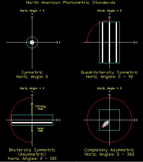
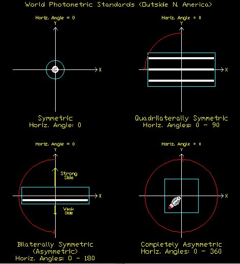
Horizontal Angles
The horizontal photometric angles that you will choose depend on the horizontal symmetric of your product. Fixtures can have four types of symmetry, as outlined in the table below. In Photopia it is important to choose the correct angle set based on the fixture symmetry because otherwise the output can become incorrect. Photopia always has data for the full 0-360 degrees, but averages down to the angle set that you choose. In the extreme case all 360 degrees are averaged together when you choose a horizontal angle of "0" only.
| Axially Symmetric | Quadrilaterally Symmetric | Bilaterally Symmetric | Completely Asymmetric | |
|---|---|---|---|---|
| Examples | Revolved Downlights | Louvered Fluorescent | "Asymmetric" Fluorescent Wallwash, Roadway | Directional Tunnel Lighting |
| Lamp Orientation | Along y axis | |||
| Outside U.S. | Along x axis | |||
| Beam Direction | Along +y axis | |||
| Horizontal Angles | 0 degrees only | 0-90 degrees | 0-180 degrees | 0-360 degrees |