Daylighting Simulation General Information
Characterizing the performance of daylighting systems via simulation allows you to consistently compare from device to device and predict device output in a consistent manner.
Skill Level
Advanced
Downloads
d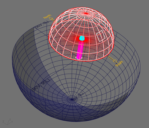
Overview
Photopia includes "lamp" models for use in modeling daylight input into devices such as skylights, light pipes, solar collectors and room windows using daylight control systems. These “lamp” models will generally be referred to as “source” models in this documentation. These source models are based on the IESNA RP-21 daylight equations that model the absolute illuminance from the sun (solar disk) at various altitude angles and the sky for various sky conditions and solar altitude angles. The sky domes include variable luminance values across the hemisphere as described in RP-21. The sun models include a 0.53 deg. spread in their beam to model the actual angular size of the solar disk, averaged over its elliptical orbit. The combination of both the sun and sky dome models produces a total illuminance onto the daylighting device area that is intended to match real outdoor conditions. Keep in mind that real conditions can vary widely and the RP-21 equations represent average conditions. Such variability is what makes consistent physical measurement of daylight devices such a challenge and is one reason why daylight simulations are desirable.
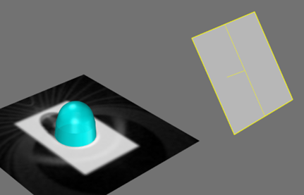
Using the daylight source models is different than using the electric lamp models in Photopia's library since the daylight source models are used to illuminate the outside of devices to get light into them rather than illuminating an optical system from within. To work with devices of various shapes and sizes, the daylight source models are setup to illuminate a particular sized area and you need to set up the appropriate size so that your device is fully illuminated. The sun models are generally square and get rotated to their appropriate solar altitude angle. Thus, they produce a distinct rectangular patch of light on a horizontal surface. The illuminance across that patch is constant and you just need to ensure that the patch is large enough to fully illuminate your device. It's also helpful to size the sun model so that the patch is not too much larger than your device. This ensures that a larger fraction of the rays generated by the source enter the device. The image below shows an appropriately sized sun model illuminating the prismatic cover dome lens of a tubular skylight. The patch of direct sunlight on the illuminance plane clearly shows the shadow of the full dome lens.
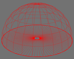
The default sky dome models are configured so that they uniformly illuminate about a 4' (1.2m) diameter area. Light spreads beyond this circular area because of the way the light is emitted from the sky dome patches, but it fades to a much lower level beyond the circular region of interest. To fully illuminate your device and maximize the fraction of sky dome rays that enter your device, this model should also be scaled larger or smaller depending on your device size relative to this 4' (1.2m) circular area reference.
Since the sun and sky dome models will produce some rays that don't enter the daylighting device, the complete model generally needs to include a shield to block stray light from being included in photometric output. Shields are discussed in more detail below.
The sun and sky dome models are provided as independent source models. Instructions for importing the models are provided in the following sections as well as other details that are important when simulating daylighting systems in Photopia. Since it's often necessary to scale source models and it can be beneficial to leverage scripting to run sets of simulations, daylight modeling is best suited to the Photopia for Rhino interface.
Shielding
Shields are required to prevent stray light the light from the sun and sky dome from being included in the photometric output of your daylighting device. Thus, the shield should have an aperture that only allows light from the sun and sky dome source models into your device and blocks all other light.
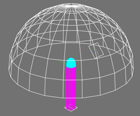
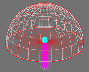
The images below show the sun and sky dome models along with a tubular skylight device. Light will enter the cyan colored dome on top of the tube. The light to be photometered emits from the bottom of the magenta colored tube. The left image shows just the tubular skylight parts and the lamp models. The right image includes a red shield, which includes a hemispherical surface offset just outside of the sky dome model and a round plane at the bottom.
Orientation
The world -Y direction is assumed to be due south, while +Y is due north. The default orientation of the sky dome models are such that the plane containing the sun is due south. Thus the sun will be in the world YZ plane, with the sun toward the -Y direction. The sun models should be rotated within the YZ plane. The sun will be in the 180° horizontal plane of the photometry. See the image below for a reference of how the sun and sky dome models are oriented with respect to the CAD world coordinate system and Photopia's default photometric coordinate system.
For circular devices such as tubular skylights, photometering the devices as bilaterally symmetric allows the azimuthal orientation of the sun to be accounted for as a rotation about the Z axis when the photometry is applied in a full room lighting analysis. If your device does not face due south or if you require the sun to be in other solar azimuthal planes, then rotate the sun and sky dome models about the world Z axis as needed and assume a completely asymmetric photometric distribution.
Importing Sun & Sky Source Models
The following information assumes that the device being illuminated (the outside elements of a skylight, for example), are centered at the CAD origin. The bottom of the device being illuminated is assumed to be at Z=0.
Sun and sky models are imported individually. The sun models are made so that they all import centered at the origin and are aimed straight down toward the world –Z axis. This default orientation is only appropriate for the 90° solar altitude sun models. All other solar altitude models must therefore be moved and rotated into their appropriate position. This can easily be done in Rhino from the Right Side View. Before rotating the sun model, move the model up above the object being illuminated with some tolerance in between the objects. The exact distance above the object isn’t critical since the sun models produce a relatively collimated beam. After the model is moved up, then rotate it about the world X-axis by the appropriate angle. For example, rotate the 30° solar altitude model by 60° about the X-axis so that it ends up 30° above the world XY plane that defines the horizon. The sun models are assigned a clear material so they can be positioned inside of the sky dome model and won’t block any of the light from the sky dome.
The clear sky domes have been made such that the sun is assumed to be in line with the –YZ plane as well. The sky dome models import with the base of their hemisphere at the origin. This is the right position if the bottom of your daylight collection device is at world Z=0. Do not rotate the sky dome unless you want to model a different solar azimuthal angle away from due south. In this case, then rotate both the sun and sky dome models about the world Z-axis as required to get your solar azimuth. A positive rotation will put the plane of the sun east of south and a negative rotation, west of south.
The sun and sky dome models are defined to be spectrally flat. The only exception being the SUN403X3-5200K model, which is the sun at a 40° solar altitude, 3' square with spectral data from 280-4000nm. The spectrum has a CCT of 5200K. The solar spectrum comes from ASTM G-173, direct + circumsolar (5° cone around the solar disk).
Sun Model Naming Convention
The sun models for clear sky use are named “SUN??XxX.LAMP” and the sun models for partly cloudy sky use are named “SUNPTY??XxX.LAMP.” In both cases, ?? = the solar altitude angle and XxX indicates the size of the model in feet. For example, SUN303x3.LAMP means it is the sun model for a 30° solar altitude and it is 3’ x 3’ square, to be used with clear sky. Solar Altitude is the angle up above the horizon, so 10° is near the horizon and 90° is directly overhead.
Sky Dome Model Naming Convention
The sky dome models are named “CLRSKY??.LAMP,” “PTYSKY??.LAMP,” and “CLDSKY??.LAMP,” where ?? = the solar altitude angle. CLRSKY = Clear Sky, PTYSKY = Partly Cloudy Sky, and CLDSKY = Cloudy Sky
Raytrace Parameters
If using only sun models in your analysis, then you can use 10 to 25 million rays for good results. Keep in mind that the larger your sun model area is beyond the size of your daylight collector, the fewer rays that will enter your device. Fewer rays means a decrease in the resolution of your output.
The sky domes are relatively large in diameter since they need to generate a relatively even illuminance over an area large enough to accommodate the daylighting device. They concentrate most of their light toward the center of the hemisphere, but some light also strays away from the center. Only that light falling near the center of the hemisphere accurately models the way light is received from the sky dome. The large diameter requires that you use a larger test distance. Photopia may not generate the correct output if you have light emanating from sources that are outside of the “photometric sphere” (which has a radius equal to the test distance). A large fraction of the light generated by the sky dome will not enter the daylighting device, so it's also important to trace a large number of rays to produce good resolution results. We recommend you use the following settings:
Raytrace Settings
Initial Source Rays: 20 to 100 million.
# of Ray Reactions: Whatever is required to fully reflect light through the device. This could be 100 or more ray reactions in tubular devices.
Photometric Output Specification
Test Distance: 45’ (15m) (This needs to be large enough so that the entire sky dome and daylighting device is within the photometric sphere.)
Intensity Distribution Angles: If you are modeling a daylight collection device with the sun in the -Y direction of the YZ plane, then the output of your device will be bilaterally symmetric which requires horizontal angles from 0° to 180°. If you rotated the sun and sky dome models to be at a different solar azimuth away from due south, then your horizontal angles will need a range of 0° to 360°.
Daylight Collector Efficiency
The efficiency shown in the Photopia report will be the ratio of the lumens collected by the photometric sphere divided by the total lumens emitted by the sun and sky dome models. As already stated, not all the light emitted by the sun and sky dome models will be incident onto the daylighting device. So the efficiency shown in the report is not likely to be meaningful for characterizing your device performance. A more appropriate measure of the device efficiency is the ratio of the lumens exiting the daylighting device divided by the number of lumens incident onto it. There are two possible ways to determine the incident lumens. One is to use Photopia to determine the total lumens that are incident onto the outer aperture of the daylight collector. The other is to multiply the horizontal aperture area of the daylighting device by the total horizontal illuminance due to the sun and sky dome. Of these two options, the second option is most commonly used and therefore the recommended method. The easiest way to determine the total horizontal illuminance onto the daylight collector is to use the daylighting calculator spreadsheet, "LTI-Optics-Daylighting-Calculator.xls.” If using the first method, then make a separate analysis where you set the material of the outside of your device to be perfectly black using the ZERO0000 reflector material. Then make a simulation using a smaller number of rays and see how many lumens are absorbed on the outer surface geometry in the Raytrace Report.
Scaling
The sky dome models have a 30’ (9.1m) radius. This produces an even illuminance over an area large enough to accommodate 4’ (1.2m) diameter devices. If you need to analyze larger or smaller devices, then you can scale the sky dome models as necessary. The default sun models are 3’ x 3’ & 5’ x 5’ (0.9m x 0.9m & 1.5m x 1.5m), so they should be scaled up or down depending on the height and width of the daylighting device. Keep in mind that the height of the device needs to be fully illuminated so the sun model needs to be tall enough when at low solar altitude angles.
Since the lumen output of the sun and sky dome models are set to produce the correct absolute illuminance over the area they illuminate, their lumen output needs to be scaled up or down as their size, and thus the area they illuminate, is scaled up or down. Their lumen values need to be scaled by the square of the size scale factor used. For example, if you make the sun or sky dome half the size, then you need to multiply their lumen values by (0.5)2 = 0.25. If you double the size of the sun or sky dome, then multiply their lumen values by 22 = 4.
Scripting
If you plan to do many simulations with different sun incidence angles, optical geometry, etc., then you should explore the Python scripting options in Rhino. All Photopia features can be scripted, including modifying geometry created with native Rhino commands, Photopia's PODT and Grasshopper. Any number of raytraces can be run in loops and any part of the output can be saved or summarized in an output file.
See the “Scripting & Optimization” section of our documentation.
An example of how this works in this video tutorial.
Leveraging this automation in Photopia for Rhino allows you to explore many more designs in much more detail than could be done manually building and simulating each design variation. When working with smaller sets of models however, it can also be helpful to run them as a group using Photopia Queue.