Contact Us
You may email support inquiries to us at the follow address: 
Should you need to call us, our support hours are 8 AM - 5 PM MST. Our technical support staff can be reached at 720-891-0030.
Support Policy
For
Technical support is only available if you have an active Annual Maintenance contract.
If your Annual Maintenance contract is expired, you can use these online resources. If you need assistance beyond these, you may renew your Annual Maintenance contract.
It is beyond the scope of standard technical support to assist you in creating optics or teaching you SOLIDWORKS or Rhino.
We offer training if you need a quick start, more detailed help, or assistance with a specific project.
Installation
Photopia for Rhino installs as an plug-in to Rhino 6, Rhino 7 or Rhino 8.
Photopia for Solidworks installs as an add-in to SOLIDWORKS 2022-2025.
Requirements
SOLIDWORKS
Requirements
- SOLIDWORKS 2022 - 2025 (works back to 2018, but not officially supported)
- Windows 10 or 11
- 64-bit Intel or AMD process (not ARM)
- 16GB RAM
- 2 GB disk space
- Internet access
Not Supported
- Windows 8 or older
- Windows Server (any version)
- ARM Processors
- 32-bit processors
Rhino
Requirements
- Rhino 6, Rhino 7 or Rhino 8
- Windows 10 or 11
- 64-bit Intel or AMD processor (not ARM)
- 16GB RAM
- 2 GB disk space
- No more than 63 CPU cores
- Internet access
Not Supported
- Windows 8 or older
- Windows Server (any version)
- ARM Processors
- 32-bit processors
Recommendations
CPU
Photopia performs all raytracing calculations on your CPU and these calculations are multi-threaded. Therefore, a faster CPU with more cores will result in faster raytraces.
Photopia can use an unlimited number of cores, however all of those cores must be on the same NUMA Node. Raytraces cannot be split between NUMA Nodes (processors) at this time.
A processor's Boost speed is typically the speed the raytracer will use if allowed based on power management and thermal considerations.
Graphics
Photopia does not perform any raytracing calculations on the graphics card.
A better graphics card will likely improve other aspects of your CAD system.
Disks / Storage
During the raytrace Photopia will write out results files and read library data from disk. For this reason, fast disk access will result in some speed improvements.
The best option is a local SSD, followed by a local HDD, followed by network storage (sometimes unreliable for SW).
Install and Setup
SOLIDWORKS
Rhino
Mac OS
The core Photopia raytrace only runs in Windows.
Although Rhino has a Mac OS native version, to use Photopia for Rhino you will have to use Rhino inside of Windows.
The best option for running Solidworks or Rhino on Mac OS is to dual boot using BootCamp (unless you have an M1 Mac, in which BootCamp isn't yet possible.
Using a virtual machine solution, like VMWare Fusion, Parallels, or VirtualBox isn't officially supported by Solidworks or Rhino, and so it may have some hiccups or performance impacts. However, we do have customers using these solutions that are happy with their performance.
Another option you have is to Remote Desktop or VNC into a Windows machine, either located in your office or hosted on a provider like AWS or Azure.
PDM/Vault SetupSOLIDWORKS Only
Photopia for SOLIDWORKS has several library files that are installed locally. This includes:
- Lamp and Material data files in %programdata%\LTI Optics\Library\
- Lamp Part files in %programdata%\LTI Optics\Library\Solidworks\Library\Lamps\
- Appearance files in %programdata%\LTI Optics\Library\Solidworks\Library\Photopia Appearances\
In order to ensure that Photopia for SOLIDWORKS functions correctly, all of the files in the above folder must remain in place.
If you operate a PDM/Vault to store, version and share files among users, Photopia can work within this system.
You could create a shared Lamps folder that user's would pull from and copy our library to this folder, however this is not recommended for Photopia users. Since we do not have all lamps as Part files yet, the "Add Lamp" function in Photopia manages this and creates part files as necessary. If you were to just put the current Part files in a folder, your users would miss out on all of the other lamps in our library. Additionally, they would not be able to edit items like lumens, watts, and mating when adding, they would have to do that as a separate step.
Our recommendation is when your users check an assembly into the vault, they should also check-in the Lamp Model Part files that are being used in that assembly. These could be put in a Lamps directory if you wish, or just stored alongside the assembly. When another user checks out the assembly, they'll get a local copy of the lamp model in that checked out folder. For any users with Photopia installed, it will still run the raytrace properly since the data is included in the part file.
Once a lamp part is in an assembly, the name and location of the part file is not critical. User's may rename and/or move the part file anywhere they wish and the raytrace will still perform as long as they still have Photopia installed.
my | photopia Online Licensing
Beginning with Photopia 2020.1 released August 2020, Photopia uses an online licensing system, MyPhotopia.
Project / File Setup
SOLIDWORKS
Analyses must be performed inside of Assembly files.
All project settings and raytrace results are stored inside of your Assembly file.
The orientation of the assembly model does not matter, Photopia for SOLIDWORKS has tools to set up the photometric test coordinates for your model.
All items are saved per configuration, allowing you to test multiple setups inside the same assembly model.
Rhino
All project settings and raytrace results are stored inside of your Rhino 3DM file.
The orientation of the model does not matter, Photopia for Rhino has tools to set up the photometric test coordinates for your model.
Rhino - Nested Blocks
IGES or STEP files exported from a solid modeler assembly file will contain multiple parts and sub-assemblies. All of the parts will be contained within nested blocks, all on a single layer when first imported into Rhino. To avoid the tedium of exploding multiple times and moving parts to layers you manually create, Photopia for Rhino includes a tool that does all of that automatically. The tool produces a new layer for each block based on the part names and maintains sub-assembly structures of the original assembly by using sub-layers. Turning off a layer in Rhino that contains sub-layers turns off all sub-layers in one click, just like turning off the display of a sub-assembly in a feature tree.
Usage:
- Import the IGES or STEP file into a new Rhino model.
- Run the ExplodeBlocksToLayers command.
- Type "L" at the first prompt to set the option for a new layer per block. The default option will put all parts onto a single layer.
- Then select the imported block and press enter.
Lamps
Lamps are special versions of SOLIDWORKS parts or Rhino blocks that have all of LTI Optics' detailed lamp model data incorporated in them. This means that when you run a raytrace you're using the full detailed lamp model, even if the display geometry is simplified. You will have accurate far and near field distribution, as well as full color data for our new color lamps. Rhino displays the exact 3D lamp model data. In SOLIDWORKS, there are two basic types of lamps you'll encounter.
Types
Full Rhino
Rhino will show the full Photopia lamp geometry, including emission surfaces. This is the actual geometry that is sent to the raytracer, and thus is polygon based.
Full SOLIDWORKS
For new lamps and popular old lamps, we'll have a full SOLIDWORKS part that shows the geometry of the lamp. This geometry is just for illustration, we use much more detailed geometry during the raytrace.
Generic Placeholder Geometry
For older lamps we'll have a simple placeholder part so that you know where the lamp is, but you won't see detailed geometry. Don't worry, we still use the detailed geometry in the raytrace, we just don't have a SOLIDWORKS representation of it.
For these lamps, the Lamp center is set at the 0,0,0 point from Photopia, which is generally the Photometric Center or center of the luminous area of the lamp. This is typically:
- Top center of the phosphor area for LEDs
- Arc center for MH lamps
- Center of tube for linear lamps
Adding A Lamp
SOLIDWORKS
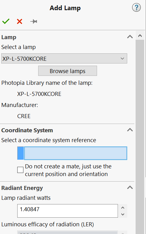
- In your assembly model, choose Add Lamp from the Photopia tab or menu.
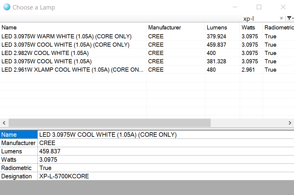
- Use the drop down to pick the lamp based on its short code, or use the Browse Lamps button to use a sortable browser.
- You may select a Coordinate System now to position the lamp, or use mates later to orient the lamp. The Coordinate System -Z will correspond to Photometric Nadir of the lamp, and +Y corresponds to a Horizontal Angle of 0deg.
- Adjust lamp lumens and electrical information as necessary.
- You can pattern/mate/move/etc the lamp part just like any other Solidworks part.
Rhino
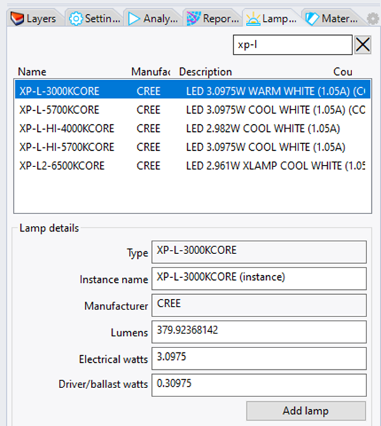
- In your model, choose Add Lamp from the Photopia menu or toolbar.
- Scroll thru the lamp list or type a keyword in the Search box.
- Click on your chosen lamp in the list.
- You may edit any of the Lamp Properties before you insert it.
- Click Add Lamp to begin placing the lamp.
- Either type in a coordinate at the command line or use the mouse to click the lamp into place.
- You may move/rotate/array/copy the lamp just as any other CAD item.
Updating A Lamp
SOLIDWORKS
- Right click on the Lamp part and choose Edit Lamp from the right click contextual menu.
- Adjust lamp lumens and electrical information as necessary.
Rhino
Within Rhino you can modify a single instance of a lamp, or all instances that you select. This makes it easy to update the lumens of all lamps at a single time.
- Select the lamp in the CAD model.
- Go to the Photopia Lamp panel.
- Adjust lamp properties.
- Click Modify selected lamp.
Using an IES file for a lamp
If your luminaire uses LEDs with off the shelf secondary optics from companies such as Ledil, Carclo, Fraen, etc. they may be represented using a special set of lamp models in Photopia's library. The special lamp models consist of planar geometry and will emit light in a distribution driven by the IES file you assign to it. The light will be emitted uniformly from the front surface of the lamp geometry. We have created a range of models that can be used for various sized optics. You will see them in the lamp list with names that begin with "LEDLENS..." The rest of the name indicates the geometry of the source, with a single number indicating a diameter. Some of these lamp models also include several copies so you can work with multiple lens types in the same luminaire. In this case, the extra copies have numbers at the end of their name. Some of these models include:
- LEDLENS20MM (This has a round emission area)
- LEDLENS50MM (This has a round emission area)
- LEDLENS75MM (This has a round emission area)
- LEDLENS19x95MM (This has a rectangular emission area for symmetric beams. It is sized for the Ledil Florence product line.)
- LEDLENS95x19MM (This has a rectangular emission area for asymmetric beams where the main throw is perpendicular to the long axis of the lens. It is sized for the Ledil Florence product line.)
SOLIDWORKS
To set the lamp model's IES file, just rename your IES file to match the model name you want to use and put it into the following folder: C:\ProgramData\LTI Optics\Library\Lamps
Note that this folder is sometimes hidden by Windows, so if you don't see it in Windows Explorer then change your Folder Options to display all hidden folders and files.
Once you load the lamp into your model, then you will set its lumens, LED watts and driver watts in the lamp properties screen to define the values appropriate for your LED, its running current, temperature and lens efficiency.
To update the IES file for your simulation, just update the IES file in the folder and re-run your simulation. The raytrace will use the latest data in the Library folder at the time you begin the raytrace.
Rhino
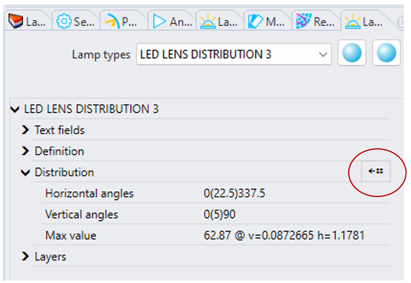
There are 2 ways to assign your IES file to a lamp model in Rhino. The first is to rename your IES file and copy it into the lamp library folder as described under Solidworks. The other option is to assign the IES file via the “Lamps editor” panel. If this panel is not already available, then you can open it by clicking on the gear icon in the upper right corner of a current docked panel and choose “Lamps editor [photopia]” from the list displayed. Select the LEDLENS… lamp model in the CAD view and then click the icon circled below in the Distribution section of the Lamps editor panel to browse to your IES file.
Once a lamp is loaded into Photopia, its IES file data is loaded into the model. The IES data is also loaded when the file is selected as described above. If you later need to change the IES file or if you’ve updated the data in the IES file, then reload the file via this import button.
LIMITATIONS
Light is emitted uniformly from the planar emission area, which is an approximation.
If you have lenses or reflectors close to the emission areas, they may not perform as they really will.
Using Rayset Data
If you don't find your lamp model in our Library, then we recommend that you use another library model of the same LED package style whenever possible. This will generally provide the best results since the Photopia lamp models create accurate ray emission points and can include the LED full spectral properties. If we don't have any models similar enough to your lamp in our library, then you can use a rayset file provided by the LED manufacturer.
In Photopia, raysets get associated with a lamp model from our library to serve as geometry that move, orient, copy, array, etc. as needed within your optical assembly. We suggest that you use simple lamp model geometry, such as our RADIMG01 and RADIMG02 models, so that the Photopia lamp geometry does not interact with the rays from the rayset. Many of Photopia's LED models include active reflector and lens geometry that will interact with rays from raysets, so these should be avoided.
Raysets might be oriented differently than you expect, so it's always best to turn on 3D rays and run a simulation with the full photometric sphere active to confirm how the model should be positioned and oriented within your optical assembly. To rotate or move the rayset, you'll just rotate and move the lamp model to which it has been assigned.
Photopia uses the lumen value defined in the lamp model property management page/panel when a rayset is associated with the lamp model. It does not use a lumen value defined inside of the rayset file. When using only rayset lamps in the optical assembly, the total # of rays should be set to the # of rays in the rayset file times the # of lamp instances.
When using multiple lamp model types with different lumen outputs, whether they are all rayset models or a mix of standard Photopia lamp models and rayset models, you need to take care about the total # of rays specified. All rays start with the same energy, so the # of rays assigned to each lamp will be a function of the ratio of their lumen outputs.
For example:
- Lamp 1: rayset lamp model assigned 100 lumens (100K ray set)
- Lamp 2: standard lamp model assigned 200 lumens
Trace 300,000 rays or any multiple of this to get the right # of rays per lamp while also emitting all rays from the rayset file. 100,000 rays will emit from the rayset while 200,000 rays will emit from the standard lamp, based on their 100/300 & 200/300 lumen ratios to the total lumens in the project.
LIMITATIONS
Rayset files contain the emission points of the rays.
There are many examples where the emission points in these files are not truly representative of the actual emission point.
Here is a summary of rayset limitations.
SOLIDWORKS
Photopia for SOLIDWORKS can use .rir formatted rayset data (grayscale based rayset data) as the emission source. To use this:
- Choose Add Lamp from the Command Manager.
- You'll need to pick a current lamp model, so we recommend using RADIMG01 or RADIMG02.
- Expand the Options section to reveal additional options.
- Click Browse to find your .rir rayset file.
- Turn on 3D rays by going to Raytrace Settings.
- Run an analysis as usual.
- View 3D Rays by clicking Show/Hide 3D rays
- Rotate or move lamp as necessary to ensure proper ray emanation points.
Rhino
See the “Modifying a Lamp Model” section below for details on assigning a rayset to a lamp model in Rhino.
Assigning a lamp to your Part geometrySOLIDWORKS Only
The following instructions describe how to create the solid part geometry for an existing Photopia lamp model.
- Import or construct the geometry of your lamp model in a new SW part file. Note that most lamp manufacturers post STEP files for their parts on their websites. The lamp model part can be in any units as long as it is the correct size.
- Move the lamp geometry so that it is centered around the part origin (0,0,0). Set up the geometry so that the center of the luminous area (the center of the chip faces for LEDs) is at 0,0,0. The geometry should be rotated so that the light emits toward the -Z direction and if you have a an array of LEDs along a PCB then orient its length along the Y axis. If you have a single emitter with geometry that isn't quadrilaterally symmetric, then load that LED into Photopia's standard CAD system and see how it is oriented with respect to Photopia's world coordinates and used that same orientation within SOLIDWORKS.
- Add a reference coordinate system and name it "Lamp orientation." This should be added at the origin of the part and match the part's XYZ axes. Do not mate this coordinate system to anything and it will insert at (0,0,0) by default.
- Set the name of the part to match the lamp model LDF file name. Note that lamp models that include reflective and/or refractive components, such as the dome lens on the Cree XM-L, will have a name that has "Core" added to what is shown in the Lamps.xls file. You can confirm the lamp model LDF name by loading the lamp in Photopia. The name will be shown in the LAMP layers and also as the text on the lamp axis layer.
- With the reference coordinate system selected, choose Add Lamp from the Photopia menu and pick the lamp model you are creating from the list to get that lamp's attributes added to this part.
- Save the part with a name that matches the lamp model LDF file name.
- Add this part file the following folder: C:\ProgramData\LTI Optics\SolidWorks\Library\Lamps
- Next time you add this lamp to a project you should see your new geometry.
Modifying a Lamp ModelRhino Only
The Lamp Editor Panel in Rhino allows you to modify more details of a lamp model type beyond its output values. The modifications will affect how rays emit from this lamp type in your project. This modified lamp type can also be saved to a .source file, which can be imported into other projects. The lamp model output parameters, such as lumens & radiant watts, are stored with each lamp instance in the project. Modifying those parameters for the lamp model type will only affect default values for new instances.
This image shows the Lamp Editor panel. The following section defines all parameters it includes.
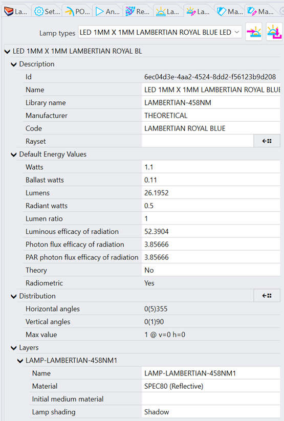
ID - An automatically generated unique identifier for the lamp type.
Name - The lamp model description.
Library Name - The name of the lamp model instances that will be used in Rhino.
Manufacturer - The lamp manufacturer.
Code - The manufacturer's lamp order code.
Rayset - Click the icon on the right side of this line to open a file dialog box. Browse to the RIR file that will define the rayset to be used with this lamp model.
Lamp Watts - The electrical watts of the source only.
Ballast Watts - The electrical watts of the ballast or driver for the lamp.
Lumens - The lumen output of the source. If no energy is in the visible spectrum, then this value should be 0. This value should also be consistent with the radiant watts and LER values, based on the lamp's spectral power distribution (SPD).
Radiant Watts - The radiant watts of the source.
Lumen Ratio - This value scales the initial radiant watt output of the source. This value allows a lamp model that includes primary optical elements such as a lens, reflector, mounting hardware, etc., to achieve the desired initial output after optical losses from those elements. This parameter therefore accounts for the optical efficiency of the lamp package. For example, if an LED loses 10% of the light from the chip after it interacts with an included primary lens & lamp base due to Fresnel reflections, TIR effects, material absorption, etc., then the lamp Lumen Ratio value would be set to 1.0/0.9 = 1.1111. When the lamp is simulated on its own, it then produces 100% optical efficiency, emitted flux = initial flux.
Luminous Efficacy of Radiation - (lumens / radiant watts). This value is a function of the source SPD. All 3 of these efficacy values can be obtained in Photopia's color report after running a power distribution raytrace for the lamp model.
Photon flux efficacy of radiation - (micro-mol-photons/second photon flux / radiant watts).
PAR photon flux efficacy of radiation - (micro-mol-photons/second PAR photon flux / radiant watts). Photosynthetically Active Radiation (PAR) photon flux is the photon flux from 400-700nm.
Theory - When set to Yes, rays will emit from the luminous surfaces of the lamp based on their relative luminance/radiance values. If this parameter is set to No, then an IES file is required to define the lamp model intensity distribution.
Radiometric - This parameter shows Yes when spectral data is provided with the lamp model.
Distribution - Click the icon on the right side of this line to open a file dialog box. Browse to the IES file that will define the intensity distribution for the lamp model.
Parameters for each lamp model layer
Name - The CAD geometry layer name.
Material - The material filename prefix for the material assigned to the lamp layer. This must be a reflective or transmissive material type. Parts of a lamp model package that include refractive materials, such as a primary lens element, are included as “non-lamp” layers in the model.
Initial Medium Material - This parameter is optional and specifies the material filename prefix for the initial refractive medium into which light emits if the emitting surfaces are encapsulated within a refractive medium other than air.
Lamp Shielding - The options are Shadow and Transmit. These define whether the geometry on this lamp layer will shadow or transmit rays emitted from other lamp layers. This parameter is optionally respected according to the “Ray Shadowing” raytrace option, which is enabled by default.
Importing and exporting .source files:
These icons on the Lamp Editor panel allow you to import & export lamp model .source files. These files are XML representations of all lamp model data. They share the same format as the lamp data written to Photopia Job Data (.pjd) files used with Photopia Queue.
Click the export icon to save a .source file to any location you choose. The filename can also be any name you choose and does not need to match the Library Name parameter.
Click the import icon to import a .source file to use in another project.
The .source files are a separate type of lamp model file from the lamps currently in Photopia's library. The .source file data is therefore edited in the Lamp Editor panel, not the Lamps panel.
Creating a Simple Lamp ModelRhino Only
You can create a lamp model in Rhino based on different shapes, spectrums and distributions. The following describes the variables that can be defined. These lamp models can be edited, exported and imported as described in the previous section. To get started, choose Photopia / Create Simple Lamp from the main menu.
Name – The lamp model name will also define the layer name on which it’s created.
Shape of lamp – The lamp shapes currently supported include Disk, Rectangle, Sphere & Hemisphere. Once a shape is selected, then you’ll be prompted for the relevant dimensions and asked to specify which surfaces are luminous.
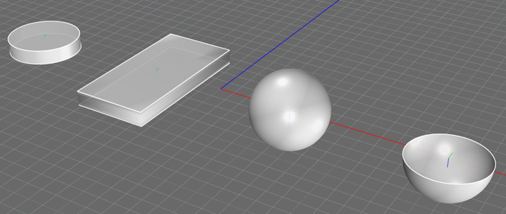
SPD – The choices are currently 458nm, 534nm, 625nm, 3000K, 4000K & 5700K.
Distribution – You can assign an IES file to the lamp or give it a “Theory” based emission. The “Theory” option assigns all surfaces an equal diffuse luminance value. This means that the surface luminances are constant for all emission angles. The resulting intensity distribution is therefore based on the luminous area exposed to each emission angle. For example, a flat disk with luminous top and bottom surfaces but no luminous sides will have a Lambertian distribution up and down. If sides are added to make a cylinder, then more light will emit to the sides depending on the height of the cylinder.
Once the lamp is created, then you can move, rotate, array, etc. as you require just like any other lamp model. To change the output, select the lamp and open the Lamps panel. Open the Lamp Editor panel to make more detailed changes to its properties.
Materials
Photopia models a wide range of material optical properties for various types of optical surfaces. The 3 general types of materials include:
Reflective - Materials that only reflect light. The reflected light can be specular, scattered or a combination, with properties varying by the light incidence angle. Reflectance properties can be defined as constant for all wavelengths or variable by wavelength. The wavelength range can be defined anywhere within the UV, visible or IR range.
Transmissive - Materials that both reflect and transmit light. The same properties defined for reflective materials can also be defined for transmitted light. Transmitted light can pass straight through a surface as a “specular” component, scatter or a have combination of both specular and scattered components. Transmissive materials are generally used to model light through diffusing lenses or lenses with repeated structured patterns such as prismatic lenses.
Refractive - Materials that model light via effects described by Snell's Law of Refraction and Fresnel's Equations. Thus, rays refract into and out of the material based on the indices of refraction of the outer and inner materials. Rays can totally internally reflect (TIR) inside of the material when incident upon the exit surface beyond the critical angle. Rays partially reflect/transmit at each optical interface based on Fresnel's Equations. Light is absorbed inside of refractors based on the material extinction coefficient. Refractive materials are generally considered to be clear (non-scattering) with smooth outer surfaces, but can include scattering properties on the outer surfaces as well as volumetric scattering from particles within the material.
Rays inside of a refractive medium are assigned an index of refraction based on the material properties and wavelength of the ray at the first ray/surface intersection when the ray enters the material. If the ray subsequently interacts with a refractive surface that's been assigned a different index of refraction, then the ray becomes invalid and is included in the “Anomalous interactions” section of the Raytrace Report. This scenario is most commonly encountered when assigning individual surfaces of a refractive part unique materials, such as a textured surface. In some cases, the base clear refractive material might contain variable indices by spectrum while the textured material assumes a constant index for all wavelengths. To avoid this problem, ensure that both the clear and textured materials use the same constant index over all wavelengths.
Reflective and transmissive material properties are measured in our own optics lab with a custom-built HDR imaging based BSDF measurement device and custom-built integrating spheres. Spectral reflectance and transmittance properties can be measured from 200 - 1100nm. The light scattering properties (BSDF data) is measured at a wide range of light incidence angles for both isotropic and anisotropic materials. The total integrated reflectance & transmittance values are also measured over a wide range of light incidence angles.
All materials that include a wavelength range in their description have properties that vary by wavelength over the specified range. Such materials should only be used with light sources that emit within the same wavelength range. All materials without a wavelength range in their description have properties that are constant for all wavelengths in a simulation. Unless a specific wavelength is indicated in the material description, the material properties are generally appropriate over the visible range (380-780nm). Refractive materials for the visible range use a single index of refraction generally measured at the sodium D-lines, 589nm, which is very close to the center of the visible spectrum.
When using spectral materials, you need to use the "Power Distribution" raytrace option. This forces the raytracer to track spectral properties on each ray. This option is more memory & computationally intensive, so it isn't the default raytrace setting when the lamp flux energy units are set to lumens. The power distribution raytrace is not required for lumen based simulations since lamp spectral lamp properties within the visible can be represented with just 3 tristimulus values. Tristimulus values are all that's required since all color metrics can be derived from tristimulus values, including RGB display values, chromaticity values, color temperature, etc. Tristimulus values aren't sufficient for modeling dispersion, wavelength conversion with phosphors, computing photon flux, etc., so the power distribution mode is required for these types of simulations.
SOLIDWORKS
Photopia for SOLIDWORKS uses the SOLIDWORKS Appearance system to assign Photopia raytrace materials to parts. This allows you to assign materials to individual faces, features, bodies or parts, and lets you use the Appearance Manager to audit which surfaces have Photopia Materials assigned as well as Display States to maintain several configurations of your material assignment.
The Solidworks apperance system can be complicated and there is a hierarchy of appearances based on where they are assigned, so it is important to understand this system. You can view the Solidworks Appearance Hierarchy Guide here.
Rhino
Photopia materials in Rhino are managed via the Photopia panel . Photopia materials are separate/unique from the Rhino materials/finishes, which means you can keep your rendering materials assigned as well as your Photopia materials.
Assigning Materials
Lists of materials are provided within each CAD interface. You can also see a fully searchable material list that includes images for many of the materials.
Material spectral properties - Unless noted in the material description, the material properties are constant for all wavelengths. Materials with variable properties by wavelength include the wavelength range they cover at the end of their description.
SOLIDWORKS
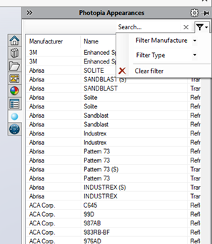
The Photopia appearances are listed under the Photopia icon on the Task Pane on the right side of the screen. You can search the list by typing parts of a name or description in the box. You can filter the list by manufacturer or type. Selecting a material will show more details at the bottom of the pane.
There are several ways to assign appearances in SOLIDWORKS:
- A selected appearance in the list can be dragged into the model and dropped onto the geometry to which it will be assigned. A flyout menu will pop up allowing you to assign the appearance to a face, feature, body, part, or part at the assembly level.
- Pre-selecting a face, feature, body, or part in the FeatureManager and then double clicking on the Photopia appearance in the list will also assign the appearance.
Photopia for SOLIDWORKS uses the SOLIDWORKS Appearance system to assign Photopia raytrace materials to parts. This allows you to assign materials to individual faces, features, bodies or parts, and lets you use the Appearance Manager to audit which surfaces have Photopia Materials assigned as well as Display States to maintain several configurations of your material assignment.
Appearance Hierarchy
SOLIDWORKS geometry can have appearances assigned at multiple levels. For example, an appearance can be assigned to a part while a different appearance is assigned to a face on that part. In this case, the SOLIDWORKS appearance hierarchy will determine which appearance is used during the ray-trace. The same hierarchy is used for renderings in SOLIDWORKS. The order of the hierarchy is listed below. Levels higher in list supersede lower levels.
Controlling appearance order:
- Component Level Assignment (part@assembly level)
- Face Assignment
- Feature Assignment
- Body Assignment
- Part Assignment
Rhino
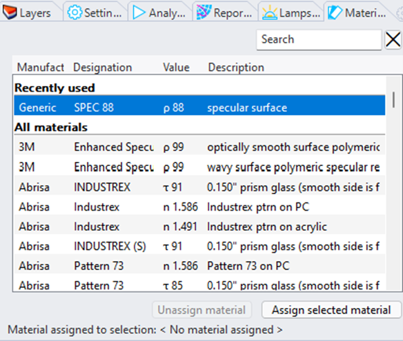
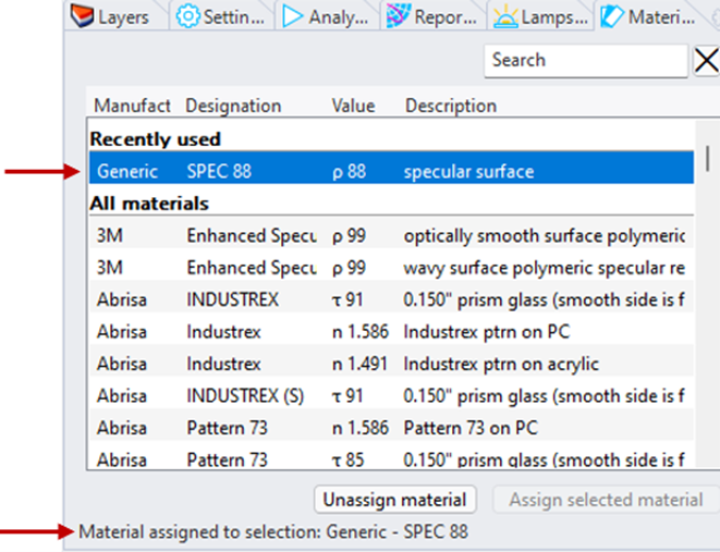
The Photopia materials are listed in the Materials panel. You can search on any part of the manufacturer, designation, or description, choose a recently used material or scroll the general list. The “Value” shown indicates the reflectance (ρ), transmittance (τ) or index (n) for reflective, transmissive, or refractive materials, respectively. This is also your indication of the material type. The reflectance and transmittance values shown are for the 0° incidence angle only.
To assign a material to model geometry:
- Select the geometry in the CAD view.
- Find the material you want in the list.
- Click the “Assign selected material” button or double click the material in the list.
Confirmation of the assignment will be shown at the bottom of this panel as well as on the command line.
Changing & Confirming Material Assignments
SOLIDWORKS
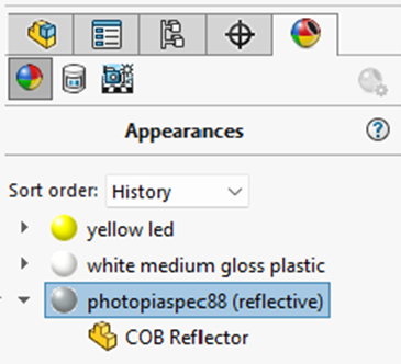
The Display Manager shows all appearance assignments in the model. Photopia appearance names are structured as “photopia + material filename.” The example below shows that the Photopia “Spec88” appearance is assigned to the “COB Reflector” part. To remove an appearance assignment, select the geometry in this tree view, then press the delete key. You can also reassign a new appearance to the same geometry to override the assignment.
Rhino
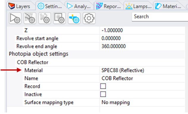
You can confirm the material assignment to geometry in Rhino by viewing the Photopia object settings in the Settings panel or by seeing what’s indicated in the Materials panel when the geometry is selected. Both panels provide a way to unassign the material or choose a new one.
Solid Model Transmissive Materials
Transmissive materials use measured BSDF data to drive the ray reactions. The measured BSDF data accounts for the effects of the full material thickness. The full reaction of the material is applied to a single ray/surface interface.
When a CAD model is constructed with solids, a lens will have a thickness and the ray will pass through multiple surfaces. Special Solid Model versions of transmissive materials have been created to avoid the full effect of the material being accounted for multiple times as the ray passes through the multiple surfaces. The Solid Model version of the material is indicated with (s) at the end of the material designation in the material list.
Transmissive materials that have unique properties for each side, such as smooth on one side and textured on the other, will have the “front side” surface indicated in the material description. The front side faces to the outside of solid model geometry. If your model requires the “back side” surface finish to face toward the incident light, then you’ll need to use the non-solid model version of the material, also referred to as the “double-sided” version. The double-sided version should only be assigned to single surfaces, not the entire solid model geometry. In SOLIDWORKS, this means assigning the double-sided material to the appropriate face of the solid part. In Rhino, it means first exploding any solid geometry to surfaces, then assigning the double-sided material to the appropriate surface.
Anisotropic Materials
Anisotropic materials are materials where there is a grain or feature that create a scattering distribution that is a function of the horizontal incidence angle. Ribbed aluminum, linear prisms and elliptical diffusers are a few examples of anisotropic materials.
In the library anisotropic materials are identified by a (A) in the name and the word "anisotropic" in their description.
Just like other materials, the first step is to assign the appearance/material to the geometry using the same steps outlined above.
The next step is to orient the material which depends on your version of Photopia.
SOLIDWORKS
- Anisotropic appearances can only be applied to faces in SOLIDWORKS. So be sure to select the face level of geometry when assigning the appearance.
- Use the “double sided” version of the appearance, i.e. the non-solid model version without the (s) designation.
- Select the same face to which the appearance has been assigned and choose "Edit appearance orientation" from the Photopia CommandManager.
- You should see arrows drawn across the polygons that make up the face. The appearance description defines the meaning of the arrow in the scatter distribution.
- You can adjust the orientation of the arrow from its default by entering a new angle. A positive value is a counterclockwise rotation. The arrows will only be shown while editing the orientation. The orientation angle displayed will reset to 0° after closing and re-opening this property management page. So you are always entering an angle adjustment from the current stored orientation.
Special considerations when working with parts in a sub-assembly:
- Ensure that the sub-assembly is “rigid” not “flexible.” Orientation data is not reliably passed to the raytracer when sub-assemblies are made flexible.
- You can assign the anisotropic appearance to the face while working either in the part or top level assembly, but you must set the anisotropic orientation direction while working in the sub-assembly that contains the part with this appearance assigned. Failing to do so could result in the face orientation data not being passed to the raytracer.
Rhino
- Select the surface to which an anisotropic material has already been assigned, then choose Photopia > Orient Anisotropic Material from the main menu.
- Enter the “Planar” option when prompted to select a mapping strategy. This is currently the only mapping strategy available in Rhino. Arrows will be drawn across the surface showing the default orientation. The appearance description defines the meaning of the arrow in the scatter distribution.
- You will then be prompted to define a rectangle that defines the orientation plane. Using the default, you can choose 2 corners. If you are orienting on a flat surface, then choose the 2 opposite corners of that surface. If you are orienting on a curved surface, then you should define a rectangular plane that allows you to best project an orientation onto the curved surface. For more details on the other rectangle definition options, see Rhino's documentation at this link ( http://docs.mcneel.com/rhino/5/help/en-us/commands/rectangle.htm ).
- Once the rectangle is defined, you can specify the angle orientation away from the default either graphically or by entering a value in degrees at the prompt. A positive angle is a counterclockwise rotation.
- Enter “A” to accept the orientation at the final prompt.
- If you want to view the arrows or re-orient the arrows on a surface, then select the surface again and start the same command. The mapping strategy now has an option for “Current” to accept the previously defined rectangle.
- The orientation direction will always be referenced to the initial 0° direction shown when the orientation was first defined. Entering the same orientation angle as previously entered will result in no change. You should enter the absolute orientation angle with respect to the initial direction.
- Orienting surfaces via their UV directions will not reliably specify anisotropic material orientation for the raytracer.
Volumetric Scattering
Beginning with Photopia 2017, Photopia supports volumetric scattering refractive materials. This is for materials which scatter light within their volume, usually via pigment or diffusion particles. These are a special class of Refractive materials, and as such require the General Refractor Module or Photopia Premium. Volumetric scattering can also be used along with spectral material properties to model phosphor particles suspended in a clear material. With a volumetric scattering material, your geometry will impact the scattering (thicker parts will scatter more).
Photopia uses a specific XML formatted file for defining the material properties. For Volumetric Scattering, the scattering is described by the Beer-Lambert Law. Photopia accounts for the extinction coefficient within the clear base material, the scattering coefficient (likelihood to scatter), the absorption of the scatter reaction, as well as the distribution and energy conversion of the scatter reaction.
Current Library materials with Volumetric Scattering are:
- Evonik Acrylite LED EndLighten 0E011 L - for 12-24" wide sheets
- Evonik Acrylite LED EndLighten 0E012 XL - for 24-48" wide sheets
- Evonik Acrylite LED EndLighten 0E013 XXL - for 48-72" wide sheets
- Generic 3000K phosphor particle in liquid silicone
- Generic 3000K phosphor particle in acrylic
- OptiColor ACC1410WT 2.5% Loading Acrylic Diffuser
- OptiColor ACC1410WT 4.25% Loading Acrylic Diffuser
- OptiColor ACC1410WT 6% Loading Acrylic Diffuser
- OptiColor ACC2170WT 4% Loading Acrylic Diffuser
- OptiColor ACC2170WT 8% Loading Acrylic Diffuser
- OptiColor ACC2170WT 12% Loading Acrylic Diffuser
- OptiColor PCC2258WT 1% Loading Polycarbonate Diffuser
- OptiColor PCC2258WT 1.75% Loading Polycarbonate Diffuser
- OptiColor PCC2258WT 3% Loading Polycarbonate Diffuser
- OptiColor PCC2393WT 1.5% Loading Polycarbonate Diffuser
- OptiColor PCC2393WT 3.75% Loading Polycarbonate Diffuser
- OptiColor PCC2393WT 6% Loading Polycarbonate Diffuser
Full details are provided in this Volumetric Scattering Documentation.
Adding a Material to the Library
If you're looking for a material that you don't find in the Library, please let us know and we'll work on adding it. Often, you may use a custom material that isn't generally available. We can add this material to a custom library for your company. For information on getting a material in the Library, please see this order form.
Modify a Material
Materials can be modified by editing the material data files in the library or by using the Material Editor. The Material Editor is currently only available in Rhino.
You can modify the integrated reflectance of reflective materials, the integrated reflectance and transmittance of transmissive materials, and the index of refraction and extinction coefficient of refractive materials. The integrated reflectance and transmittance values can be changed as a function of incidence angle. You can also change the ratio of the specular component to the scattered light for both reflective and transmissive materials. You cannot edit the material BSDF data.
Material Editor (Rhino Only)
The optical properties of materials are generally defined by one or more library files associated with the material. When materials are assigned to geometry in your model, the material properties are read from the library when the raytrace is run. If you choose to edit material properties in Rhino, a copy of the library material will be made and kept within the Rhino model. The material data files in the library will not be changed. This ensures that they will perform as expected for other projects that reference them.
To edit a material in Rhino, you first need to “import” the material data into the Rhino model. Go to the Material panel, select the material that you want to edit, then click on “Advanced” to expose the “Import material” button. Clicking this button imports the material properties. You will now see “Recently used,” “Internal materials,” and “All materials” listed in the Materials panel when the Search box is cleared. The word “internal” will be added to the default material designation to differentiate it from the version in the library.
You can assign internal materials to your geometry just like any other material, by selecting the geometry in the CAD view and then double clicking the internal material name you want to use.
Internal material properties are edited in the Material Editor panel. If it isn’t already opened in your Photopia Panel layout, then add it by clicking Rhino’s gear icon on the panel group, then “Show panels...”
Select the internal material to edit from the drop-down list at the top of the panel. There’s also a button to remove the selected material from the model if you no longer want to use it.
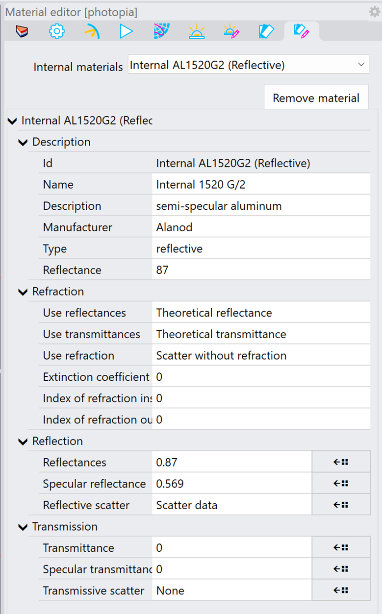
The image above shows the parameters that can be edited. All values under “Description” are for reference only and won’t affect the material performance. The “Reflectance” shown for this reflective material is generally just the first number in the .RFL file that describes the reflectance as a function of the incidence angle, but is shown for reference purposes only in the description.
The parameters listed under Refraction, Reflection & Transmission are relevant depending upon the material type being edited. In this case, only the values in the Reflection section are used. Note that both the Reflection and Transmission sections are used for “Transmissive” materials.
The values shown in the “Reflectances” and “Specular reflectance” text boxes are the average values read from the data files that define these values as a function of incidence angle. These are the .RFL and .RSC files. The following section describes all library material file formats in more detail. If you enter new values into these text boxes, then they’ll be used as constants for all incidence angles. Otherwise, you can import new data from files you create with the icon on the right of each row.
You can import new .BRD and .BTD BSDF data files in the “Reflective scatter” & “Transmissive scatter” parameters.
The Refraction section parameters are:
Use reflectances – Options for “Theoretical reflectance” and “Use reflectance data.” The theoretical option means that Fresnel’s Equations are used. You can override these default values if you are using an AR coating for example. In this case, the .RFL data in the next section will be used if you choose “Use reflectance data.”
Use transmittances – The same as described above, but applied toward the transmitted refracted ray reaction.
Use refraction – When scattering is added to the refracted ray reactions, you have the option to scatter around the refracted ray direction or an undeviated ray direction.
Extinction coefficient – This value is in 1/inches.
Index of refraction inside and outside of the refractive medium.
Material Data File Formats
The material file descriptions are as follows:
Reflective Material Files:
Filename.rfl - ASCII file of integrated reflectance values at each incidence angle. Files can contain an arbitrary angle set, so long as 0, 90 and 180 degrees are included. 0° is the front side of the material. Valid reflectance values range from 0.0 to 1.0.
Filename.brd - Binary file of the BRDF data for a material. This file cannot be modified. A .brd file only 2 bytes in size indicates the material is specular.
Filename.rsc - ASCII file specifying the ratio of the reflected light that is reflected in a specular manner. Note that these are not the specular reflectance values, but the fraction of the reflected light that is specular at each angle. To derive specular reflectance from these values, multiply these values by the reflectance at each incidence angle. Valid values range from 0.0 to 1.0. This file may or may not be associated with a material. A data byte indicating whether or not the material has a specular reflectance component is contained in the .brd file.
Transmissive Material Files (includes reflective files above, plus the following):
Filename.trn - ASCII file of integrated transmittance values at each incidence angle. Files can contain an arbitrary angle set, so long as 0, 90 and 180 degrees are included. Valid transmittance values range from 0.0 to 1.0.
Filename.btd - Binary file of the BTDF data for a material. This file cannot be modified. A .btd file only 2 bytes in size indicates the material is clear or image-preserving.
Filename.tsc - ASCII file specifying the ratio of the transmitted light that is transmitted in a straight-through manner. Note that these are not the straight-through transmittance values, but the fraction of the transmitted light that passes through un-scattered at each angle. To derive straight-through transmittance from these values, multiply these values by the transmittance at each incidence angle. Valid values range from 0.0 to 1.0. This file may or may not be associated with a material. A data byte indicating whether or not the material has a straight-through transmittance component is contained in the .btd file.
Refractive Materials Files:
Filename.rfc - ASCII file containing 3 values: the index of refraction of the outside medium (usually assumed to be air at 1.0), the index of refraction of the material averaged over the visible spectrum, and the extinction coefficient in units of inches. Note that the extinction coefficient is applied in the equation: Trans = e^(k*L), where e is the exponential (2.71), k is the extinction coefficient, and L is the distance the ray travels in the material in inches. Thus, k is a value per inch. If you need to create special materials that have the same index on both sides of the surface to change ray states from being inside or outside of a refractive medium without having any ray reaction at the surface, then you'll need to set the 2 indices to be different by at least 0.00011. Making the difference smaller than this treats the indices as equal, which is a special case where the raytracer ignores the optical interface. An example file for an air/air interface would be:
1.0 1.00011
0.0
Spectral Material Files:
The spectral data for reflective & transmissive materials are defined in several different files. The .spdrfl & .spdtrn files include an incidence angle, multiplier and reference to a spectral matrix file (*.spdmatrix) on each line. The multiplier scales all values in the .spdmatrix file. The spectral reflectance & transmittance is defined in a matrix, where each row is an input wavelength, and each column is an output wavelength. For materials that don't shift wavelengths, all reflectance/transmittance values are shown for each wavelength along the diagonal of the matrix. All other values are 0. The first 3 values in the matrix file define the wavelength range as start, end, increment in nm. Wavelength increments can't be less than 1nm at this time.
The first 3 values in the .spdrfc refractor material files define the start, end and wavelength increment in nm. The remaining lines include the outside index, inside index and extinction coefficient for each wavelength.
Spectral materials also require a .material file.
To Modify Material Files:
You can modify any of the ASCII files described above with a text editor such as Notepad. Follow the instructions below to create a new version of a file without changing the original copy:
- Go to the C:\ProgramData\LTI Optics\Library\Materials folder in Windows Explorer. Be sure you are viewing the file extensions. If you don't see the ProgramData folder listed, then be sure that all hidden files and folders are being shown in Explorer.
- Find a material that has all of the same general characteristics as the new material you wish to create. For example, pick PAINT001 if you want a reflective material that has a specular component.
- Copy all of the files for the original material to files with a new filename of your choice. The filename prefix should not include spaces.
- Modify the data in the files as you require.
- The material lists shown in Photopia are read from .lib files. The default .lib files for the various material types are named Reflect.lib, Transmit.lib & Refract.lib file. Since these files are updated whenever Photopia is installed, any custom materials should be listed in unique .lib file names. So make a copy of the .lib file you need depending on your material type. Rename the filename prefix while preserving the original name that describes the type. For example, rename Reflect.lib to be Reflect_YourCompany.lib. These files are ASCII files, so open the new .lib file in Notepad. There are 5 entries on each line, with each data item separated by a tab character. The data is: manufacturer, designation, description, value (either 0° percent reflectance, 0° percent transmittance, or index of refraction), and material filename prefix. Modify the data on the first line of the file to represent your new material. Delete the remaining lines in the file. You can now add any number of new materials to this file later.
- Save and close the .lib file. The next time you open Photopia in SOLIDWORKS or Rhino, your new material will be listed.
Recording Planes & Recording Objects
Photopia has 2 types of recorders that collect flux density onto surfaces, recording planes & recording objects.
Recording planes are flat, rectangular surfaces that only collect light incident onto one side. Since their geometry is limited to flat rectangles, their grid resolution can be defined, and all grid values are available to view in the results. Geometry used to define recording planes can't also be optically active as a reflector or lens surface.
- only planar rectangular surfaces
- are not optically active (must not have a Photopia material assigned)
- records incident energy on front only - 1 channel
Recording objects can be made for any reflector or lens optical surfaces in the model. Unlike recording planes, these surfaces can have any shape or curvature and must be optically active. The flux density is recorded on all mesh polygons of recording objects for incident and exitant light, for both the front and back sides of the object surfaces. So there are 4 sets of data (channels) for recording objects.
- any surface shape (not necessarily flat or planar)
- are optically active (must have a Photopia material assigned)
- records incident and exitant on front and back - 4 channels
Create Recording Planes
SOLIDWORKS
- Select a planar rectangular face in your model. It is important that the face be planar, rectangular, and not already assigned a Photopia Appearance.
- Click "Add Recording Plane" from the Photopia CommandManager tab.
- Define the grid name and description.
- Confirm the Lower Left Corner of the plane, or shift as necessary. The lower left corner defines how the grid data will be displayed in reports.
- Confirm the plane direction. The front side of the plane is indicated by a blue arrow. Recording planes only collect light onto their front side, so the arrow should face toward your light source. Flip the orientation if necessary.
- Define the grid resolution by entering either column/row spacing or the number of columns/rows.
You can also check a box for “Enable fluence mode,” which converts the grid so that it collects “fluence rate” values rather than illuminance/irradiance values. Fluence rate is the total flux incident onto a sphere divided by the sphere cross-sectional area. The spheres are centered in each grid patch and have a diameter equal to the grid spacing. Fluence rate is a more useful metric of flux density for applications such as air and water disinfection where particles are equally affected/dosed by flux arriving from any direction. Fluence rate values multiplied by time of exposure in seconds equals “fluence,” which is the dose onto particles. Fluence rate has units of watts/area while fluence is joules/area.
Rhino
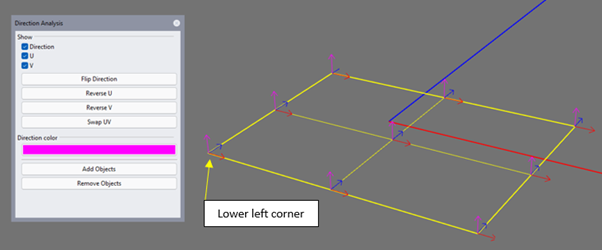
- First, confirm your planar face is oriented properly. The surface orientation can be checked and flipped with Rhino's “Show object direction” tool on their Surface Tools panel, or by typing "DIR" at the Command Line. The lower left corner is indicated with the red and blue U and V direction vectors as shown below.
- Select a planar rectangular face in your model. It is important that the face be planar, rectangular, and not already assigned a Photopia Material.
- Click "Add Recording Plane" from the Photopia toolbar.
- Enter a plane name at the Command Line.
- Confirm the grid resolution at the Command Line.
In order to record Fluence select the plane and then go to the Photopia Object Settings and check the box for "Fluence Mode" which converts the grid so that it collects “fluence rate” values rather than illuminance/irradiance values. Fluence rate is the total flux incident onto a sphere divided by the sphere cross-sectional area. The spheres are centered in each grid patch and have a diameter equal to the grid spacing. Fluence rate is a more useful metric of flux density for applications such as air and water disinfection where particles are equally affected/dosed by flux arriving from any direction. Fluence rate values multiplied by time of exposure in seconds equals “fluence,” which is the dose onto particles. Fluence rate has units of watts/area while fluence is joules/area.
Modifying Recording Planes
SOLIDWORKS
- Select the surface/face in the CAD view.
- Right click and select the Recording Plane icon from the flyout menu.
- Change any of the desired parameters
Recording planes in SOLIDWORKS get their size and location from the surface at the time they are defined. If the surface is later moved, resized, or deleted, the change won’t be recognized by the recording plane. So if you need to modify a recording plane, then click the “Delete all recorders” button. Modify your surface and then redefine your recording plane and any other recorders in the model.
Rhino
- Select the surface/face in the CAD view.
- Go to the Photopia Object Settings panel. Pre-selecting the recording plane isolates the properties for the plane.
- Here you can also enable "Fluence mode".
The recording plane is associated with the surface used to define it, so if that surface is transformed or deleted, the recording plane will recognize the change.
Viewing Recorders
You can view recording planes & recording objects by choosing Results and then the Illuminance Planes / Recording Planes tab, or turning on their display in the Model view using the Recorder Display On/Off button.
Creating recording objects
recording objects allow you to view the light interacting with any object in your model. The object surfaces must be optically active, so they need to have a reflective, transmissive or refractive material assigned to them. If you don't want the object to impact the light in your model, you can assign the CLEAR001 transmissive material.
SOLIDWORKS
- Select one or more faces or objects in your model. It is important that you select the same level of geometry to which the Photopia appearance was assigned. So if the appearance was assigned to a face, then select the face, not the full part that includes the face. If you created a “Convert to mesh body” feature, then select that in the FeatureManager.
- Click "Add Recording Object" from the Photopia CommandManager tab. There is an option to enable or disable the recording object in this screen in case you need to make this change later.
- After a raytrace is complete, click on the "Show/Hide recorders" button in the Photopia CommandManager to display all recorders in the CAD view.
- The "Recording surface settings" button on the Photopia CommandManager tab allows you to specify the way the recorders are displayed. See information below for more details.
The recorder mesh resolution is set by default by the Image Quality settings in SW, under Settings > Document Properties. Slide the top bar labeled Shaded and draft quality HLR/HLV resolution into the red zone for a finer mesh. More detailed options are available in SW2018 and later by adding "mesh body" features to your part geometry. This is done in your part by choosing Insert > Surface > Convert to Mesh Body… You are then prompted to select a body from the part. If a body represents a solid, then a single mesh will be made that represents all faces of the solid. If you want to create separate meshes for each face, which is helpful when viewing surface statistics (max, min, average, ...) in the recorder report or when you need to assign a unique appearance to one face of the part, then you should build the model geometry from surfaces rather than solids. You can then select the surfaces from the list of bodies to convert to a mesh. Be sure that you also assign the Photopia appearance to the mesh feature and select the mesh feature before clicking the "Add Recording Object" button.
If you need to convert a solid part into multiple surfaces, then you can use the SW tools to create zero offset surfaces and delete original solid faces.
- Choose Insert > Surface > Offset...
- Select the face and enter 0 as the offset distance. Hide that face.
- Choose Insert > Face > Delete.
- Select the face that was just used to create the offset surface. Be sure the "Delete" option is selected.
- Then show the offset face.
This results in 2 surface bodies rather than a single solid body.
Rhino
- Select one or more objects or surfaces in your model.
- Assign a Photopia material if you have not done so already.
- In the Photopia Settings panel , click the "Photopia object settings button."
- Find your object/surface and check the "Record" box. If you first select your object in the CAD view, then it will be isolated in the list.
- After a raytrace is complete, click on the "Show/Hide recording surfaces" button on the Photopia toolbar to toggle the display of the recording surfaces.
- The "Recorder display settings" button in the Photopia Settings panel allows you to specify the way the recorders are displayed. See information below for more details.
- The Recording object mesh resolution is set with the "Mesh parameters" button on the Photopia toolbar.
Recorder Display Settings
SOLIDWORKS
Rhino
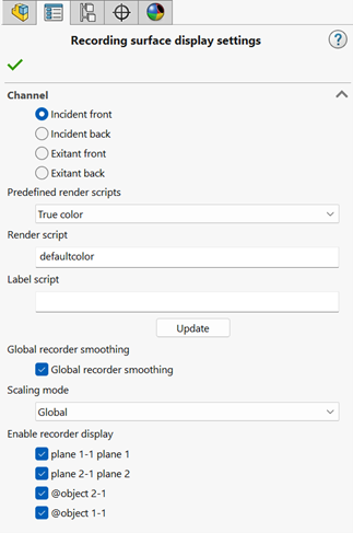
Predefined Render Scripts: Render Script Presets allow you to select from a default set of display settings, including: false color, true color, grayscale, spectral shifts for non-visible wavelengths and a range of options for color uniformity.
Render Script: Once a preset render script is selected, then the render script will be displayed in a separate box. All values of that render script can then be edited to manipulate the recorder display even further.
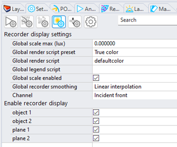
Global Max: By default, all recorders will be scaled to the global max value found on all recorders. The global max is automatically found when the "Global scale max" parameter is set to 0 in Rhino. You can enter any other value there if you prefer.
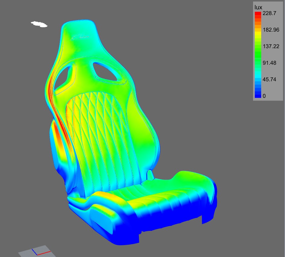
Legend: A legend is displayed when using global scaling and viewing gray scale or false color plots. If you uncheck the "Global scale enabled" box in Rhino or switch to local scaling in SW, then each recorder will be scaled according to its own max value. A legend can't be displayed in this case since the same colors will represent different magnitudes. When global scaling is used, the value of red on the legend is based on both the max value found on all recorders as well as the area over which that max is achieved. If the max is only on a very small area, indicating “noisy” results, then red will be assigned to a lower value to allow then colors of the legend to represent more of the data on the recorders. The true max value will be shown to the upper left of the legend display.
Global Recorder Smoothing: The "Global recorder smoothing" option determines whether or not the data on each patch is blended with neighboring patches. Smoothing the data makes a more realistic looking image of the light pattern. If you turn off the smoothing, then you see the raw data in each patch of the recorder.
Channel: This allows you to view any of 4 data sets on the surfaces. The channels are the incident light onto the front and back sides of the surfaces as well as the exitant (emitted) light from both the front and back sides. All 4 channels are available for recording objects, but only on the front incident light channel is available for recording planes.
Enable Recorder Display: The display of the individual recording planes and objects can be set in this section. Checked items are displayed when the recorder display in the CAD view is toggled on. This list is a function of the selected channel. Recording planes only include data for the “incident front” channel, so they will only be listed when this channel is selected.
Viewing Color Differences
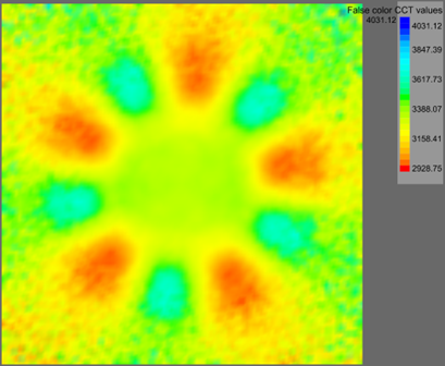
Color differences on recorders can be viewed subjectively with the True Color script or objectively with a range of color metrics as described below. These plots complement the true color plot when color differences in the light pattern are subtle and provide quantitative values that are helpful when the beam needs to meet specific color uniformity requirements.
False color CCT values: This plot allows you to view CCT variations in the beam pattern. This false color plot will show black when the CCT is outside of a “reasonable” range. This range is defined in the render script and can be changed if desired. CCT values are computed from the tristimulus values at each recorder patch. These values will get noisy with very low or zero light levels, typical in the beam fringe or outside of the beam pattern. Values outside of a defined “clipping range” are therefore shown in black. In the default scripts shown below, CCT is clipped at 2000K at the low end and 16000K at the high end. Change those values in both scripts to change the “clipping” range.
Global render script: falsecolorclipped(cct(2000, 16000, 0,0), max(displaymincct, 2000), min(displaymaxcct, 16000),…
Global legend script: cct(2000, 16000, 2000,16000)
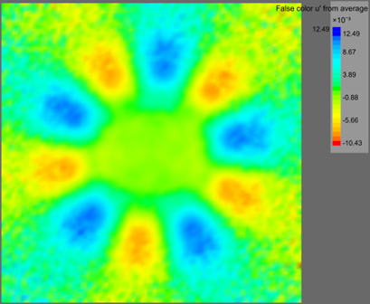
False color u’ from average: This plot shows color differences in the u’ direction in the uniform u’v’ color space.
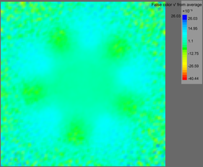
False color v’ from average: This plot shows color differences in the v’ direction in the uniform u’v’ color space.
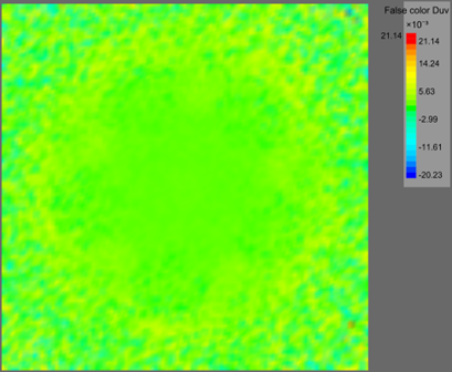
False color Duv: Duv values are the distance above (+) and below (-) the black body curve in the u’v’ color space. Despite the name of this metric, the values are computed in u’v’ and not the uv color space.
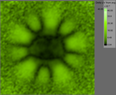
Delta u'v' from average: This plot allows you to view quantitative color differences in the uniform u'v' color space. In this color space a value of 0.001 is 1 MacAdam ellipse, which is a just perceptible color difference. Beam color uniformity requirements sometimes specify an allowable range in this color space, such as 0.004 or 4 MacAdam ellipses. In this plot, black is 0 and bright green is the highest delta u'v' value on the plane.
Photometric Settings
You'll need to tell Photopia how to orient your Photometric Coordinate System before raytracing. You'll basically be defining what is 'up/down & forward/back, which should be the same orientation as the test.
SOLIDWORKS
You first need to create a Reference Coordinate System that defines the location and orientation of the “photometric coordinate system.” The -Z axis of this reference coordinate defines the 0-degree vertical angle and +Y defines the 0-degree horizontal angle in a Type C photometric coordinate system. The origin defines the photometric center. See more details in the sections below.
Select the reference coordinate system and then click the Photometric Settings button on the Photopia CommandManager. This will automatically mate the photometric coordinate system to the reference coordinate system. This will create a new virtual part in the assembly when this property management page is closed.
You can modify the orientation & location of the photometric coordinate system by modifying the properties of the reference coordinate system to which it is mated.
Rhino
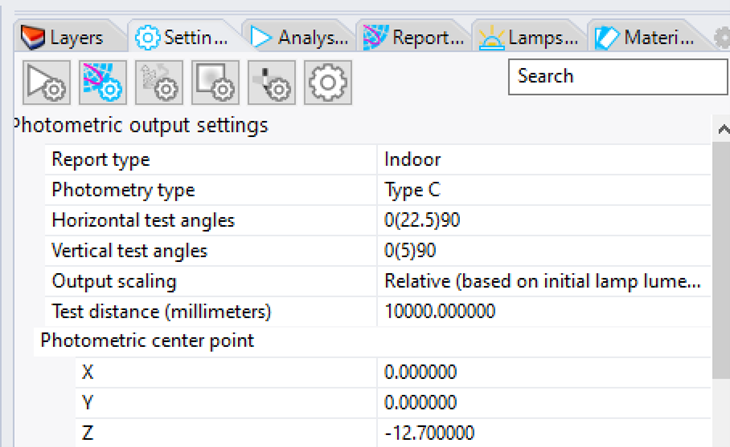
Click the toolbar button for the Photometric Output Settings
You can visually confirm the location & orientation of the photometric coordinate system by clicking the Show/Hide Photometric Sphere icon on the Photopia toolbar.
Descriptions of all settings are provided in the sections below. A few that are specific to Rhino are provided here.
Photometric Nadir The direction of a vector toward the horizontal and vertical angles of 0 degrees. Generally, the direction of the beam center. This defaults to the world -Z axis.
Photometric Azimuth The direction of the 0-degree horizontal angle. This defaults to the world +Y axis.
Manufacturer If a value is provided, then this will be included as a keyword in the IES file.
Luminaire Description If a value is provided, then this will be included as a keyword in the IES file.
Catalog Number If a value is provided, then this will be included as a keyword in the IES file.
Report Type - This selection affects the default photometric coordinate system type as well as the default photometric report that shows relevant data for the various applications. A wider range of reports is available in the Reports view in SolidWorks and in Photopia Reports.
Photometry Type - The photometry type defines the orientation and angle references of the spherical coordinate system. The appropriate type to use depends on your application. The diagrams below show the “direct” half of the photometric sphere and how it’s aligned with the reference XYZ coordinate system. This will be the “reference coordinate system” in SolidWorks and the world coordinate system in Rhino by default. The rings and ribs in the “photometric web” are defined by the horizontal and vertical angular resolutions. The shaded region shows the angles that will be included in the photometric report. The data is averaged within the hemisphere based on the beam symmetry. Note that the CAD preview of the photometric sphere shown in SolidWorks and Rhino is scaled based on the size to the model geometry rather than shown at its actual size based on the specified test distance.
Type A
The standard coordinate system for automotive, aerospace, and marine lighting devices. Photometric requirements for devices in these industries define min and max intensity values at various angles in this coordinate system. The horizontal and vertical angles can be referred to as “X” & “Y” in some standards. The beam center is generally in the direction of travel and is oriented toward the 0X, 0Y (0H, 0V) directions.
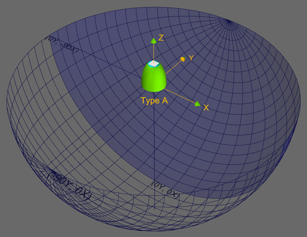
This image shows horizontal angles of (-90(10)90) & vertical angles of (0(5)90). The specific angle sets selected depend on the angles at which required intensity values are defined. Certain report types that check for beam compliance with a standard will list the required angle sets. Horizontal angles can range from -180 to +180 degrees. Vertical angles can range from -90 to +90 degrees.
For aerospace applications where light can emit in all directions around a device, you will orient the +Z axis of the reference coordinate system in the aft direction and +Y toward the sky. The full range of horizontal and vertical angles should be used, generally H: (-180(5) 180), V: (-90(5)90).
Type B
The standard coordinate system for outdoor floodlights and sports lighting.
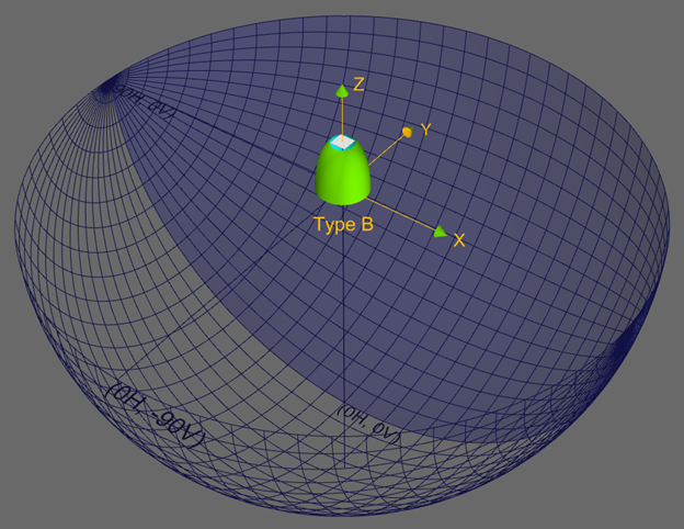
This image shows horizontal angles of (-90(5)90) & vertical angles of (0(5)90). Horizontal angles can range from -90 to +90 degrees. Vertical angles can range from -180 to +180 degrees, but most of these types of luminaires do not have any “indirect/back” light, so the vertical angles will range from -90 to +90 degrees.
Type C
The standard coordinate system for indoor and outdoor area & street lights for architectural lighting.
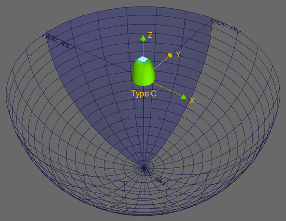
This image shows horizontal angles (designated as “L” for lateral) of (0(15)90) & vertical angles of (0(5)90). Horizontal angles are also sometimes represented by the Greek letter psi and referred as the “C plane” in Europe. Horizontal angles can range from 0 to 360 degrees. Vertical angles can range from 0 to 180 degrees. Vertical angle references include “V”, the Greek letters theta and gamma. “C-gamma” is the common European reference to the Type C coordinate system.
The angular resolution is specified between the start and end angles, e.g. (0(5)90) defines an angle set that starts at 0, increases in 5-degree increments, and ends at 90. The smaller the angular increment, the more rays you need to trace to resolve the increased resolution of the distribution. Use finer angular increments when the intensity distribution has narrow peaks or valleys. Use larger increments when the distribution is wider and smoother. In general, we recommend that the horizontal angular increment be kept at 15 degrees or less and the vertical increment at 5 degrees or less.
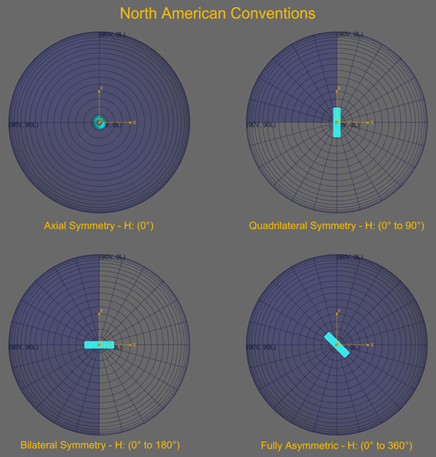
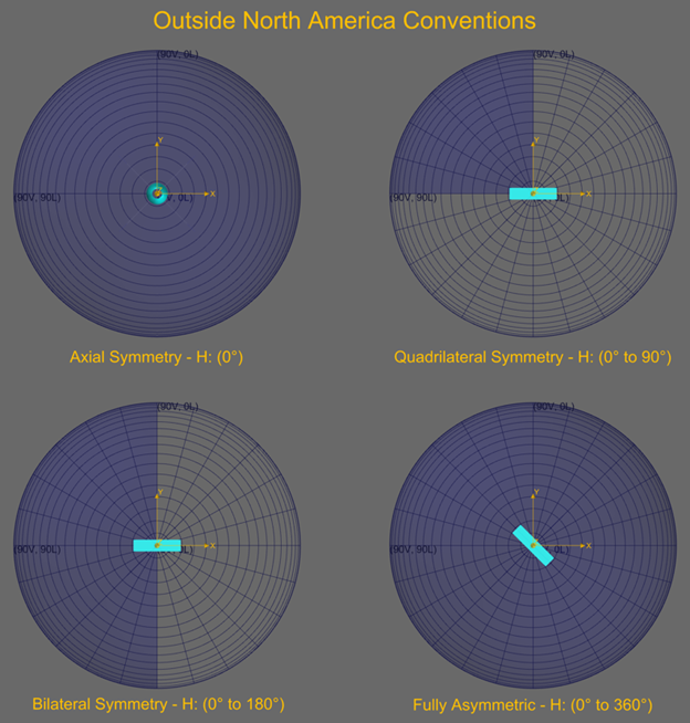
It’s best to use the minimum range of angles required to fully describe the beam, accounting for the beam symmetry. The angle sets will then indicate the type of luminaire distribution and you will get the smoothest intensity distribution with the fewest rays as Photopia will average data over the different quadrants. The vertical angle range options include:
- Direct: 0 to 90 degrees
- Indirect: 90 to 180 degrees
- Direct/Indirect: 0 to 180 degrees
There are 4 beam symmetry options for the horizontal angle range as shown in the next 2 images. These show the luminaire orientation with respect to the photometric coordinate system, with different conventions for quadrilateral symmetry in North America compared to the rest of the world. Bilaterally symmetric distributions should orient the strong side of the beam toward the 0-degree horizontal plane.
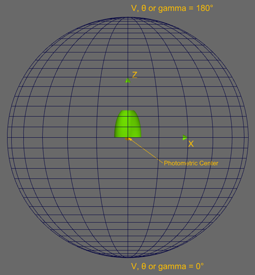
Photometric Center - The center of the photometric coordinate system should be placed at the center of the luminous emitting area of the device. If the device emits all light from a horizontal opening, such as the bottom of a reflector, then the photometric center should be placed in the center of that opening, as illustrated in the image showing the vertical angles above.
Test Distance - The radius of the photometric sphere. If you have physical photometry done, then this should match the test distance of the physical goniophotometer you are using. For “far field” photometry, the test distance should be set to at least 5 times the max luminous dimension of the device. For better results, that should be increased to 10 times. Better results means that the intensity distribution is less sensitive to the exact test distance used.
Luminous Dimensions - The luminous extents in X, Y & Z dimensions of the device. X, Y & Z with respect to the reference coordinate system. The default option will use the CAD model extents to determine these dimensions. It’s generally best to override that default with more appropriate values that represent the actual area from which the light emits. Devices that emit all light out of a horizontal opening, such as the bottom of a reflector, should set the luminous Z to 0. In architectural lighting, the luminous dimensions are important since they affect the size of the luminaire emission area in lighting application software as well as the values in the luminaire luminance & UGR tables.
Output Scaling
Relative - All output will be based on the lumens or radiant watts defined for the lamps in the model. The reports will show the optical efficiency of the model as the ratio of the output lumens/watts to the input lumens/watts.
Absolute - All output will be based on the lumens or radiant watts defined for the lamps in the model. The reports will be treated as a physical “absolute photometric” test where the lamp input lumens or watts is not known. Therefore, the reports will not include the optical efficiency. The IES file will show -1 for the lamp lumens.
Per Thousand Lamp Lumens - The total input lumens or watts into the model from all lamps will be scaled to be 1000.
Decimal Precision - The decimal precision used for the intensity values saved to the IES and EULUMDAT files. Be mindful of this setting if you have a device with very low lumen or radiant watt output.
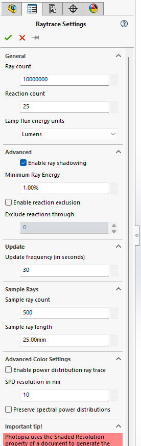
Raytrace Settings
This screen allows you to modify the parameters that control all aspects of the raytrace process. The following sections provide a description of each of the parameters.
SOLIDWORKS
Rhino
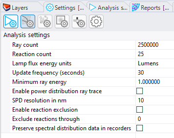
Ray Count
Specifies the number of rays for the raytrace, emitted from all sources combined. The more rays that are traced, the more refined the results. The default of 2.5 million is generally sufficient for initial results.
Each component of the results will resolve at a different number of rays.
Below is the order in which items typically resolve.
- Optical Efficiency (~50,000 rays)
- Intensity Distribution (~2,500,000 rays with 5deg vertical angular resolution)
- Recording Planes (~10 to 25 million rays at 100x100 grid size)
- Color Difference (~100+ million rays)
Reaction Count
Specifies the number of ray reactions to trace. Each ray intersection with an optically active surface is a ray reaction. The default of 25 is generally sufficient for most light to emit from or diminish within an optical system. The “Reached interreflection limit” value in the “Anomalous interactions” section of the “Raytrace Report” indicates how much light was still interacting within the optical system due to this limit. It's generally best to set the reaction count high enough so that only a small percentage of the light reaches this limit. Light pipe/light guide designs or refractors with volumetric scattering particles generally require much higher values, such as 100+ ray reactions.
Lamp Flux Energy Units
The simulation can be run with the lamp output defined in lumens, radiant watts, photon flux or PAR photon flux. Lumens are appropriate for all lighting applications for which photometric output is required. Radiant watts provides radiometric output for applications such as optical sensors, UV curing and disinfection. Photon flux or PAR photon flux are most commonly used for horticulture applications. Both "Photon flux" and "PAR flux" are based on the lamp output in micro-mol photons per second. Photosynthetically Active Radiation (PAR) flux limits the results to only wavelengths between 400-700nm. Most horticulture applications require the use of PAR flux.
When you are using lamp models that include their full spectral details, then the lamp output can be defined in lumens, radiant watts, photon or PAR flux. They are all linked by the lamp SPD, so entering output in any of these units automatically updates all of the others. If you only know the lamp output in lumens based on the LED datasheet and power parameters for example, then you can enter the output in lumens even if you want results in PAR flux. Just be sure to set the lamp flux energy units in the raytrace settings as you require before the raytrace is run. Photopia does the proper conversion from radiant watts to photon flux at every wavelength of the SPD in the intensity distribution and on irradiance planes. So you can mix any combination of white and colored LEDs and get the right PAR flux values, for example. It is important that the SPD for the lamps you choose from Photopia's library match your actual LEDs if you will be relying on the right conversion from lumens or radiant watts to PAR flux. Entering your LED output in PAR flux directly avoids the need for an exact SPD match, but the LED output in PAR flux is not always provided on datasheets.
Ray Shadowing
Used for ray generation, this ensures that lamp parts which shadow the emission are taken into account. Leave checked for the most accurate results.
Minimum Ray Energy
If a ray's energy falls below this setting, it will no longer be traced through the system. This helps speed up a raytrace by reducing time spent on insignificant rays. The amount of light lost in the raytrace due to this limit is reported in the “Anomalous interactions” section of the “Raytrace Report.”
Exclude Reactions
Enabling this option allows you to remove any number of initial ray reactions from the output, starting with ray reaction 0. This allows you to isolate any part of the output by the ray reaction number to more clearly see “higher order” effects and help isolate their cause. For example, if you have a reflector design that emits both direct and reflected light, you can isolate the beam created from the reflector by removing the 0th ray reaction from the output. You enter the Exclude reactions through value, which would be 0 in this example. Note that some LED models include optically active components such as a primary lens, so in this case your “exclude through” number would need to be increased to account for the ray reactions within the LED package.
Update Frequency (seconds)
Specifies how often the output will be updated as the raytrace progresses. The analysis status view will show the # of rays and percent complete with each update.
Power Distribution Raytrace
This option enables the full spectral data to be tracked with each ray. This is the most general way of tracking ray properties, but results in a slower ray trace since more data is processed with every ray reaction. When running a lumen based simulation that does not use any materials with spectral properties, you can leave this option disabled and all spectral properties will be converted to tristimulus values. Thus only 3 extra parameters are tracked & processed on each ray, resulting in a faster ray raytrace with less memory and storage. Tristimulus values are all that's needed to compute all color metrics including the true color recorder images. If the lumen based simulation includes spectral materials, which are indicated with their spectral range shown in their description, then you need to enable the power distribution raytrace for those material properties to be used. For example, if you want an acrylic lens to use an index of refraction that changes by wavelength, then choose the ACRYLIC1 material with a description of “standard clear acrylic (250-2800nm)” and enable the power distribution option.
All radiant watt or photon flux simulations automatically enable the power distribution raytrace since their output requires the full spectral ray data.
When a power distribution raytrace is enabled, you can also specify the resolution in nm. A finer resolution might be needed for models that include narrow band features in their lamps and/or materials. The finer the resolution, the more data tracked on each ray, and thus the slower the raytrace and the larger the memory requirements.
Preserve Power Distribution Data
This option refers to the spectral power distribution data stored with recorders. When a power distribution raytrace is run, all spectral data can be stored for each patch of every recorder in the model. This data is needed if you will be using any of the render display scripts that remap the spectrum for visualization purposes. For example, if you plan to remap UV wavelengths into the visible range so that you can view the recorders in a way similar to true color displays, which show both color mixing and irradiance magnitude in the same display. Having the full spectral data available for such display options is helpful, but it also requires more memory. This is OK for a few recording planes at their default resolution, but can become a burden on system resources when you have large recording objects with hundreds of thousands of polygons, especially since recording objects store 4 channels of data for every polygon. So it's best to leave this option off unless you specifically need the spectral remapping feature for recorder display visualization.
Sample Ray Count
The number of rays that you want displayed in the CAD view. The default of 0 results in no displayed rays. When you do want to display rays, we recommend a fairly low number such as 500 so that you can more clearly see the general ray trends. Using too high a number fills the screen with so many lines that it can be difficult to see their interactions with the model geometry. You may need to use a higher number however, when filtering the rays to see how they react with specific optical components in the model.
Sample Ray Length
The length of the ray after its last interaction with any optical components in the model, including recording planes. This value can be changed after the raytrace in Rhino and the ray display will update.
Sample Ray Filtering
For each sample ray, Photopia keeps track of several properties of that ray, including the objects that it interacted with. This allows you to filter the sample rays to display only the rays that fit a specific criteria.
SOLIDWORKS
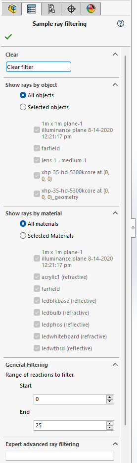
Click the Filter sample rays button on the Photopia CommandManager to open the following PropertyManagement page.
Show rays by object - Display rays that interact with all objects in the model or only those you select. Note, “farfield” is the far field photometric sphere. It’s listed as both a material and an object.
Show rays by material - Display rays that interact with all materials in the model or only those you select.
Range of reactions to filter - Defines the start and end ray reaction numbers to display.
Expert advanced ray filtering – - You can type a list of ray reaction numbers to show. The numbers do not need to be consecutive. Use a space between each value.
Invert filter - Inverts the current filter setting so all rays that were not being displayed are now displayed while the filtered rays are not.
Filtered Ray Color - Specify the filtered ray color in the box just after Invert filter. The red, greed & blue values are specified from 0 to 1, separated by spaces.
Rhino
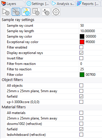
Click the Sample Ray Settings button in the Photopia Settings panel to view the screen.
Sample ray color - Set the color of the unfiltered sample rays. To change the color, click on the color designation, then click the drop-down arrow in the cell and choose a color on the pop-up dialog.
Exceptional ray color - Set the color of exceptional rays. These are rays that were stopped in the raytrace due to the problems listed in the “Anomalous interactions” section of the “Raytrace Report.”
Filter enabled - Check this option to view the filtered rays as defined by the following settings. When unchecked, all sample rays are displayed.
Display exceptional rays - Check this option to display the exceptional rays.
Invert filter - Inverts the current filter setting so all rays that were not being displayed are now displayed while the filtered rays are not.
Filter from reaction - The start reaction number of the rays displayed.
Filter to reaction - The end reaction number of the rays displayed.
Filter color - Set the color of the filtered rays.
Object filters - Display rays that interact with all objects in the model or only those you select. Note, “farfield” is the far field photometric sphere. It’s listed as both a material and an object.
Material filters - Display rays that interact with all materials in the model or only those you select.
Saving Sample Rays as CAD Entities
SOLIDWORKS
The filtered rays can be saved to a 3D sketch in the assembly. If you want to save all rays to the sketch, then keep the default filter settings that show ray reactions with all objects & materials. When finished defining the filter settings, click the Save filtered rays to sketch and close button at the bottom of this PropertyManagement page. A new 3D sketch will be created to store the filtered rays. If you want to separate different sets of rays into different 3D sketches, then define a new filter and click the same button when closing this PropertyManagement page.
Rhino
Choose Photopia > Save 3D Rays from the main menu. This will save the 3D rays displayed with the current filter settings to the current layer. If you want to save different sets of rays to different layers, then change the filter settings and current layer as desired.
Mesh Resolution
The Photopia raytrace engine uses a meshed representation of your CAD model geometry except where native geometric objects are specifically supported. Most geometry created in Rhino and Solidworks are NURBS surfaces & solid bodies, not meshes, so they must be converted before raytracing. This conversion is handled automatically when you start a raytrace, but you might need to override the default meshing for parts with fine details.
Mesh resolution is more critical in models with smoothly curved reflector and lens surfaces that have specular or clear lens materials assigned. Models with diffusing surfaces are much less sensitive to the model mesh resolution. For smooth reflector and lens surfaces, we recommend setting the Maximum Angle deviation from the surface normal to 1 or 0.5 degrees.
For recording objects, we recommend using the Maximum Element Size and Max/Min Edge Length to set your desired cell/patch size.
SOLIDWORKS
There are 2 ways to control your model mesh resolution In Solidworks. The default method is to use the model “Image Quality” resolution. This generally provides enough control, but if you need more then you can create a “Mesh Body” feature. Both options are defined in more detail below.
To view the meshes that will be used by the raytracer, click the “Show/Hide mesh preview” button on the Photopia Command Manager. This runs the first part of the raytrace process that extracts the raytrace geometry from the assembly model. The raytracing of that geometry won’t be run, but extracting the geometry might take a few seconds or a few minutes depending on your model complexity. You can watch the progress of this process in the Analysis Status window.
Image Quality
This setting can be applied in your Part files or at the Assembly level. The SolidWorks documentation indicates that the part settings will be used unless the "Apply to all referenced part documents" option is checked in the Image Quality settings screen in the assembly. Our own testing has shown inconsistent results, however. The most consistent trend observed was that the last setting defined was used, whether at the part or assembly level. When the model mesh resolution is critical to your results accuracy, we therefore strongly recommend that you view the mesh preview.
- Choose Tools > Options > Document Properties > Image Quality
- Find the Shaded and draft quality HLR/HLV Resoultion section
- Pull the slider control into the red zone for the finest mesh.
Mesh Body
- Open the Part file, or edit the Part within the assembly.
- Choose Insert > Surface > Convert to Mesh Body ...
- Select the Body to convert
- Update the resolution settings, we suggest setting the Maximum Angle Deviation and Maximum Element size.
- Click check and you'll see the new mesh
- Assign the Photopia Appearance to this Mesh Body. Delete any appearance assignments to other levels of this same geometry.
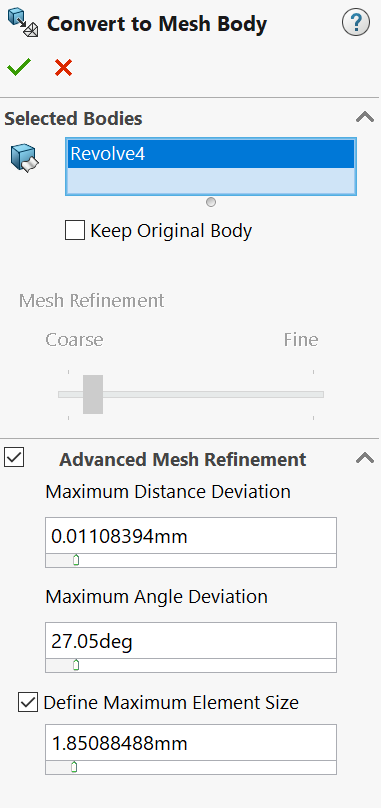
Rhino
In Rhino, click on the Photopia Mesh Settings.
You can adjust any of the parameters and then click Preview to see the mesh for your model.
Any setting kept at 0 will be non-controlling.
Maximum edge length and Maximum Angle are the two most useful settings.
See Rhino’s documentation ( https://docs.mcneel.com/rhino/7/help/en-us/documentproperties/mesh.htm ) for more details about these mesh parameters.
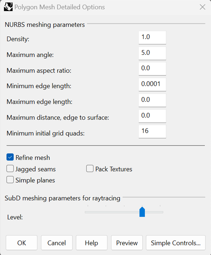
By default, these parameters will apply to all surfaces in your model that are assigned Photopia materials. This is indicated with the *custom Mesh Parameters setting in the Photopia Object Settings panel. Select one or more surfaces/objects to see this setting. If you require different mesh settings on some surfaces in your model, then choose another option from the drop-down list. Options with names such as “5mmX5mm” indicate mesh settings with minimum and maximum edge lengths set to 5mm. These “square” grid mesh options work well for object recorders, especially those with an extruded shape. Keep in mind however, that Rhino does not subdivide meshes along the extrusion direction of an “extrusion” entity. So if your surface was created with the extrusion tool, then Explode it first, so that it’s a “surface” entity.
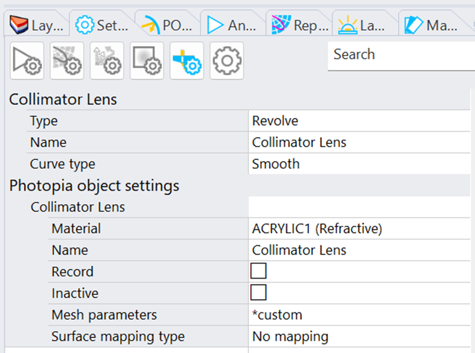
Non-critical model geometry can be set to the “Coarse0.5” option, which creates a medium density mesh with Rhino’s Density setting to 0.5.
There is no preview option when assigning mesh settings to surfaces this way, so you can confirm the mesh appearance by using the PhotopiaExtractMesh command. Select a surface and then run this command. Its simulation mesh will be created and stored on the current layer. Once you’ve confirmed the mesh details, then select this mesh and delete it. The mesh will be created from the original surface when you start the raytrace.
View Results
Results can be viewed either in the SOLIDWORKS window, Rhino panel or in Photopia Reports. This allows you to view several outputs at the same time. To view results, click the Results button on the Solidworks CommandManager or click the Results panel in Rhino.
In Solidworks the results are saved per configuration, so a single assembly model can include the results for various design options.
A wide range of photometric, radiometric & colorimetric results are shown in specialized reports & plots. Reports are generally oriented toward specific industries, such as architectural lighting, automotive, aerospace, horticulture, disinfection, etc.
See our glossary for an explanation of specific types of results.
The TM-30 color reports show a range of plots that require the full spectral power distribution rather than just tristimulus values. You will therefore need to choose the “Power distribution raytrace” analysis setting to view any of the TM-30 color reports. We recommend using an SPD resolution no greater than 10nm.
Intensity distribution data can be saved to standard IES & EULUMDAT file formats. In Solidworks, choose either of these file options in the left bar of the Results screen. Then click the export icon in the upper right corner of the screen. In Rhino, click the "IES/LDT" icon in the upper right corner of the Reports panel.
You can also view the Analysis Status during a raytrace.
Parametric Optical Design Tools
The Parametric Optical Design Tools (PODT) create reflector and lens geometry based on how you want to control the light. The parameters for the various types of optics define both the physical size and aiming properties of the design. These tools are useful when you are designing a reflector or lens that needs to produce a particular beam pattern. The optical design tools allow you to define the range of angles over which the light is directed as well as how much light is directed toward each angle in the beam. Thus, they allow you to tailor the beam intensity distribution.
Reflector Design Tool Overview
The reflector design tools create reflector profiles based on aiming light toward a range of angles or toward a range of points. Using “aim by angle” creates a reflector built from a set of parabolic sections. Using “aim by point” creates a reflector built from a set of elliptical sections. As an example, consider a reflector that aims all light toward a single angle at the beam center, creating a very narrow beam pattern. This reflector is a single parabola that collimates light as shown below when revolved into a parabolic surface:
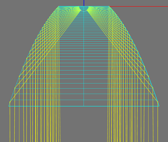
The aiming angle in the reflector above is toward the 0° vertical angle in the reflector's intensity distribution. Now consider changing the aiming angle to be 20° away from the beam center, as shown below. This is still a single parabolic profile, but the profile has been rotated by 20° about its focus. Revolving this profile about the beam central axis (a vertical line), results in the reflector shown below. Whereas the reflector aimed toward 0° would create a narrow beam intensity distribution, the reflector aimed at 20° would produce beam pattern with a spike 20° off center.
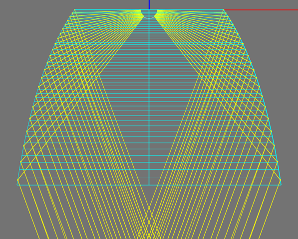
The parametric reflector design tools allow you to aim light toward any number of angles in your beam pattern, which results in a set of parabolic profiles all joined together. Combining 0 and 20 into a single reflector looks like this.
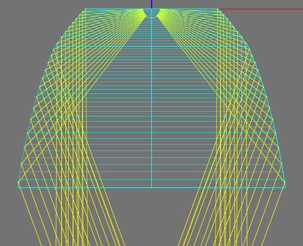
Simulating these 3 reflectors with an LED at the focus results in the following intensity distributions.
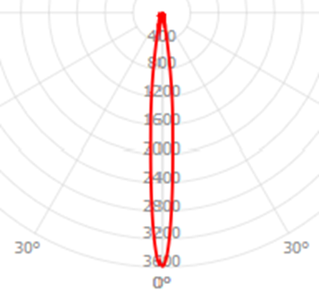
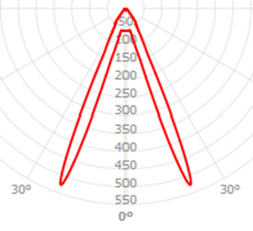
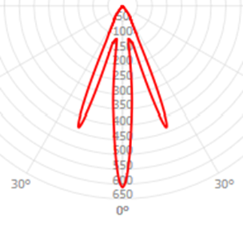
The relative intensity values at 0° and 20° in the 3rd beam are determined by how much of the reflector is allocated to each of the 2 parabolas. More specifically, each parabola gets some fraction of the total reflector angular extent. The total angular extent is the angular sweep about the focus from the bottom to the top of the reflector. In this case, it’s about 53°.
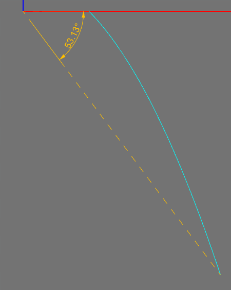
The reflector above with sections aimed at both 0° and 20° allocated 40% of the total extent to 0° and 60% toward 20°. Changing that allocation to 20% / 80% results in the following intensity distribution.
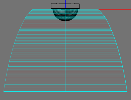
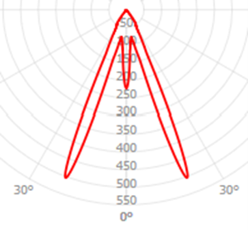
Since less of the reflector is collecting and redirecting light from the LED toward 0°, the intensity in that direction is reduced relative to the intensity at 20°. So in addition to the parametric reflectors allowing you to define the range of angles over which the reflector is aimed, they also allow you to manipulate the fraction of the reflector aimed toward each angle in the distribution. This is done by assigning a set of “weighting factors” to each reflector “aiming section.”
The reflector below shows a more realistic design, with aiming sections ranging from 0° to 20°, every 1° in between. This reflector is therefore comprised of 21 parabolic profiles all joined together. The weighting factors (WF’s) were defined so that they created a beam with a peak in the beam center that tapered off toward the wider angles in the distribution.
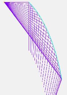
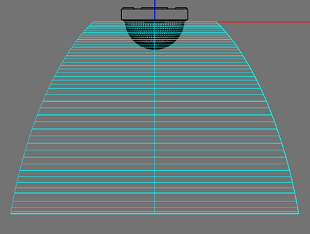
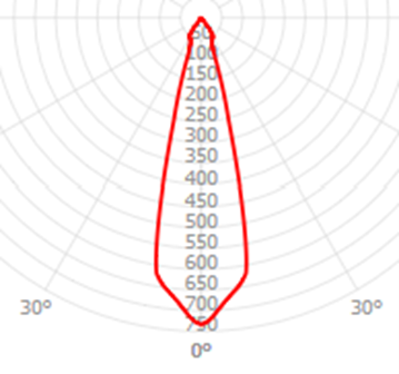
The image below illustrates the geometric input parameters for a reflector, including +/- angular conventions. The Lamp Center is the focus of the optic, the Nadir Direction defines the beam center, and the Start Point defines the fixed end of the reflector. The start point can be set at the top or bottom of the reflector. The Angular Extent defines the total angular size of the reflector. The “end point” of the reflector floats along the angular extent cutoff line with a location based on the profile shape, which is driven by the aiming parameters.
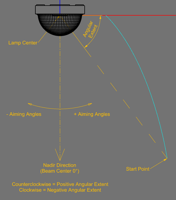
The aiming method is selected as “by angle” or “by point.” When using “by angle,” the angular conventions are as defined in the above image. When using “by point,” you enter the absolute points in the sketch or construction plane. Aiming angles are defined for each end of the reflector, with an Aiming Angle Increment that determines the total # of reflector sections between the 2 extremes. Aiming points are defined for each end of the reflector, with the Number of Points used to define the total # of reflector sections
Creating a Reflector
SOLIDWORKS
The parametric reflector will be created in a part document. A parametric reflector profile can be created in any sketch plane. If you want to create a profile so the light is aimed along the world Z axis, in line with the default lamp model orientation, then create a new sketch in the Top Plane. Once the sketch is created, then some initial geometry needs to be added to define the geometric constraints of the reflector. These include the Lamp center, Start point and a construction line that defines the 0° aiming angle. You may want to use the sketch origin as the lamp center. Add a Point to define the location of the start point. Add a construction line to define the 0° aiming angle. This is often a vertical line anchored to the sketch origin.
Once the input sketch geometry is created, select Photopia > Design Reflector and reference the geometry from the sketch in the various input parameters. The Angular extent is a parameter that could not be easily referenced, so this value is manually entered. You can determine it in your sketch via a smart dimension before starting the design tool.
Reload - This keeps a reference to reflector parameters that have been defined. Most often you only create 1 profile for a given sketch, but if you create multiple then they will be referenced in this list. This drop-down list is most often used to select the parameters to associate with a feature created from the sketch after the profile is completed.
Lamp Center - Select a point that defines the lamp center, the focus of the aiming parameters.
Start Point - This defines the start point of the reflector. This is the fixed end of the reflector and can be at the top or bottom of the profile.
Angular Extent - The full angular extent of the reflector, measured about the optical center and beginning at the start point. CCW is a positive angular sweep, CW is negative.
Edge for 0° aiming angle - Select the construction line that defines the 0° aiming angle, generally the beam center.
Aim by direction / Aim by point - Select the aiming method and define the aiming angles or aiming points.
Target Feature - A feature based on this profile does not exist at the start, so leave this reference blank. It will be referenced after the profile is added to the sketch and a feature is created.
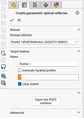
Name - Enter a name for the profile when you will be using multiple PODT profiles to create Swept, Lofted or Boundary Boss/Base features. For example, if you have 3 profiles that will drive a lofted boss/base feature, then name them Profile 1, Profile 2 & Profile 3. This allows you to easily select the appropriate PODT parameters from the “Reload” drop down list when modifying the properties of any of the profiles. The Reload list will add a unique identifier based on the date & time to each entry as seen in the example above, so choose the one for your desired profile closest to the bottom of the list when making changes.
Clear sketch contours - Check this option when you will be using multiple PODT profiles in different sketch planes to drive Swept, Lofted or Boundary Boss/Base features. When this option is checked, any non-construction geometry will be deleted from the sketch before the new PODT profile is added. When this option is unchecked, the new PODT profile is added to any geometry already existing in the sketch, including previous versions of the PODT profile.
Open the PODT Window - This button will open the PODT window where you can adjust all reflector properties.
Advanced - - Includes the “Create TIR Profile” option, which encloses the reflector profile sketch to create a solid mass of material when revolved or extruded. Otherwise, the profile created by this tool is a single curve that is generally revolved into a thin shell, as shown in the left image below. The right image shows the revolved feature created from the “TIR Profile” option that includes lines connecting the reflector curve to the central revolve axis. This is useful when using the reflector design tool to design TIR lens optics.
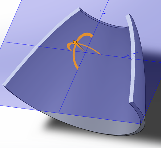
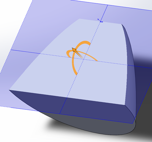
Rhino
A reflector profile can be created in any construction plane. The Front View is often used when creating a reflector aligned with the default photometric coordinate system. Once you've selected your construction plane, then click the “Design reflector” icon on the Photopia toolbar and follow the command prompts for the input parameters.
Lamp Center - The focus of the reflector aiming sections. Often the origin of the construction plane.
Aiming nadir - The direction of the beam center and 0° aiming angle. This is often in line with the -Y direction. Hold down shift and drag your mouse down to indicate a direction straight down.
Start Point - The start point of the reflector. This is the fixed end of the reflector and can be at the top or bottom of the profile.
Angular Extent - The angular sweep of the reflector can be selected with the cursor or a value can be entered. CCW is a positive angular sweep, CW is negative.
Type of aiming - Enter “D” for Direction or “P” for Point.
Aim by direction / Aim by point - Select the aiming method and define the aiming angles or aiming points.
Aiming start, end & increment - For aim by direction. Enter the desired aiming parameters.
Aiming start, end & aiming section count - For aim by point. Enter the desired aiming parameters.
Choose to open the PODT dialog or skip it. If skipped, the reflector profile will be added to the current construction plane. To edit the profile parameters, select the profile and click the “Design reflector” icon again. This will open the PODT dialog.
Reflector PODT Window / Dialog
All the parameters of an optical profile can be viewed and modified in the Solidworks PODT window or the Rhino PODT panel.
SOLIDWORKS
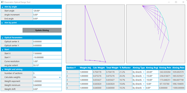
Rhino
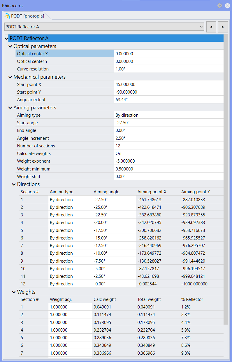
Aim by angle - The aiming angles for the start & end of the reflector as well as the angular increment between the 2 extremes. The angles are measured from the nadir direction. Click "Update Aiming" to apply changes.
Aim by point - The start & end aiming point locations within the sketch/construction plane coordinate system, as well as the number of points in between. Click "Update Aiming" to apply changes.
Optical center X/Y - The focus of all reflector aiming sections in the sketch/construction plane coordinate system.
Start X/Y - The start point of the reflector in the sketch/construction plane coordinate system.
Curve resolution - The angular resolution of the polyline profile used to approximate the parabolic or elliptical reflector sections. The curve resolution defines the angular sweep about the optical center, starting from the beginning of each aiming section, at which vertices of the polyline profile are obtained. To get a reflector profile that closely approximates the parabolic/elliptical profiles, use a small value such as 0.5° or 1°. To create a “faceted” reflector profile, use a larger value. To create a single facet for each aiming section, use an angle that is larger than the size of all aiming sections, such as 90°.
Angular extent - The full angular extent of the reflector, measured about the optical center and beginning at the start point. CCW is a positive angular sweep, CW is negative.
Number of sections - The number of aiming sections determined by the aim by angle or aim by point parameters. This value can be overridden if you need to add or subtract sections from what the aiming parameters defined.
Calculate weights - A value of “On” enables the use of the weighting factor (WF) equation.
Weight exponent - Exponent in the WF equation. A higher positive value directs more light toward wider angles. A lower negative value directs more light toward the beam center. A value of 0 sets all WF’s to the minimum value.
Weight minimum - Sets a minimum WF value in the nadir (0°) direction.
Weight shift - Shifts the angle in the cosine function of the WF equation. Useful when your beam is directed toward a surface that is not centered about the nadir direction. For example, when illuminating a vertical wall with a ceiling mounted luminaire, using a weight shift of 90° produces a more useful trend in the WF’s.
Weight adjustment - An adjustment factor that can be applied to the calculated weights for each aiming section.
Lens Design Tool Overview
The lens design tool shares the same aiming and weighting factor parameters as reflectors, but uses refraction instead of reflection to redirect the light. Because lenses/refractors control light differently, they require different geometric constraints.
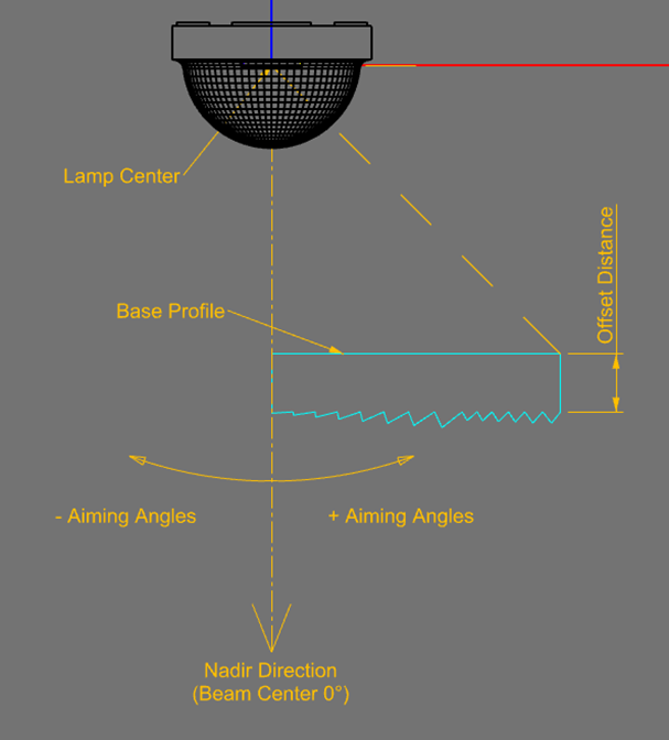
Whereas reflector shapes are determined by their aiming parameters, lens shapes are more flexible and generally defined by the style of the optic. For example, the prisms shown in the image above could be “mapped” to the flat “base profile” shown or a curved “base profile” like shown below depending on the style of the optic. The same type of aiming can be defined for either “base profile,” but the prism geometry will vary depending on shape of the base profile. To accommodate different styles of optics for any given application, the “base profile” is one of the input parameters.
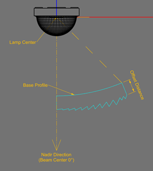
Lens designs also require a material index of refraction and the material thickness since the light will refract through 2 surfaces. All lenses start as prismatic profiles as shown in these images. Once the initial lens definition is created, a larger range of parameters are available to modify in the PODT window, as described in the following sections.
Creating a Lens
SOLIDWORKS
The parametric lens will be created in a part document. A parametric lens profile can be created in any sketch plane. If you want to create a profile so the light is aimed along the world Z axis, in line with the default lamp model orientation, then create a new sketch in the Top Plane. Once the sketch is created, then some initial geometry needs to be added to define the geometric constraints of the lens. These include the Base profile, Lamp center, and a construction line that defines the 0° aiming angle. You may want to use the sketch origin as the lamp center. The base profile can be any type of open curve. Add a construction line to define the 0° aiming angle. This is often a vertical line anchored to the sketch origin.
Once the input sketch geometry is created, select Photopia > Design Lens and reference the geometry from the sketch in the various input parameters.
Reload - This keeps a reference to lens parameters that have been defined. Most often you only create 1 profile for a given sketch, but if you create multiple then they will be referenced in this list. This drop-down list is most often used to select the parameters to associate with a feature created from the sketch after the profile is completed.
Lamp Center - Select a point that defines the lamp center, the focus of the aiming parameters.
Base profile - Select the curve that defines the base profile.
Prism steps - The minimum number of prism steps along the profile. This value is overridden by the # of aiming sections defined since each aiming section requires at least 1 prism along the profile, so keeping the default value is generally recommended.
Index of refraction - The index of refraction used to determine all prism/curvature computations based on the aiming parameters.
Minimum thickness - Minimum distance between the inner and outer lens profiles.
Edge for 0° aiming angle - Select the construction line that defines the 0° aiming angle, generally the beam center.
Aim by direction / Aim by point - Select the aiming method and define the aiming angles or aiming points.
Target feature - A feature based on this profile does not exist at the start, so leave this reference blank. It will be referenced after the profile is added to the sketch and a feature is created.
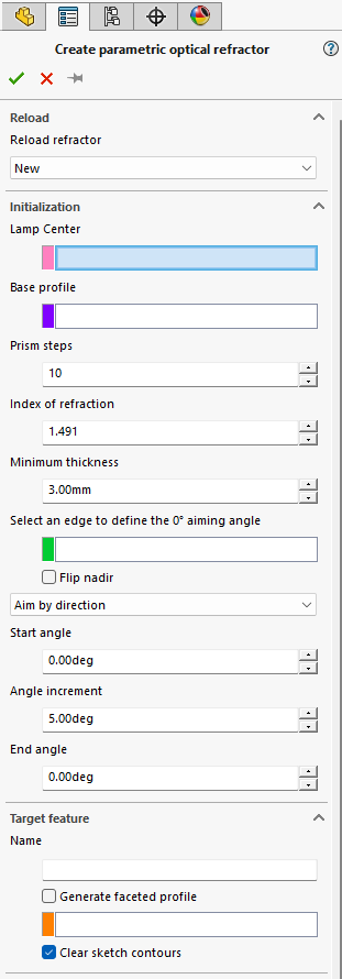
Name - Enter a name for the profile when you will be using multiple PODT profiles to create Swept, Lofted or Boundary Boss/Base features. For example, if you have 3 profiles that will drive a lofted boss/base feature, then name them Profile 1, Profile 2 & Profile 3. This allows you to easily select the appropriate PODT parameters from the “Reload” drop down list when modifying the properties of any of the profiles. The Reload list will add a unique identifier based on the date & time to each entry as seen in the example above, so choose the one for your desired profile closest to the bottom of the list when making changes.
Clear sketch contours - Check this option when you will be using multiple PODT profiles in different sketch planes to drive Swept, Lofted or Boundary Boss/Base features. When this option is checked, any non-construction geometry will be deleted from the sketch before the new PODT profile is added. When this option is unchecked, the new PODT profile is added to any geometry already existing in the sketch, including previous versions of the PODT profile.
Open the PODT window - This button will open the PODT window where you can adjust all lens properties.
Advanced - Non-editable coordinate feedback.
Base profile curve resolution - Before prism angles can be computed for the specified range of aiming angles, the base profile curve is converted into a polyline, comprised of straight line segments between a number of control points along the curve. The resolution/smoothness of the polyline is defined by a “Curve resolution” parameter. This defines the angular sweep about the focus to each new control point along the base profile curve. This parameter is a global setting in SOLIDWORKS, defined in Tools > Photopia > General Settings > Advanced > Curve resolution.
Rhino
A lens profile can be created in any construction plane. The Front View is often used when creating a reflector aligned with the default photometric coordinate system. Once you've selected your construction plane, then draw your Base profile. The base profile can be any type of 2D open curve in this plane. Once the curve is drawn, the select it and click the “Design lens” icon on the Photopia toolbar and follow the command prompts for the input parameters.
Lamp Center - The focus of the lens aiming sections. Often the origin of the construction plane.
Aiming nadir - The direction of the beam center and 0° aiming angle. This is often in line with the -Y direction. Hold down shift and drag your mouse down to indicate a direction straight down.
Prism count - The minimum number of prism steps along the profile. This value is overridden by the # of aiming sections defined since each aiming section requires at least 1 prism along the profile, so keeping the default value is generally recommended.
Index of refraction - The index of refraction used to determine all prism/curvature computations based on the aiming parameters.
Lens minimum thickness target - The minimum distance between the inner and outer lens profiles.
Type of aiming - Enter “D” for Direction or “P” for Point.
Aim by direction / Aim by point - Select the aiming method and define the aiming angles or aiming points.
Aiming start, end & increment - For aim by direction. Enter the desired aiming parameters.
Aiming start, end & aiming section count - For aim by point. Enter the desired aiming parameters.
Choose to open the PODT dialog or skip it. If skipped, the lens profile will be added to the current construction plane. To edit the profile parameters, select the profile and click the “Design lens icon again. This will open the PODT dialog.
Lens PODT Window / Dialog
All the parameters of an optical profile can be viewed and modified in the Solidworks PODT window or the Rhino PODT panel.
SOLIDWORKS
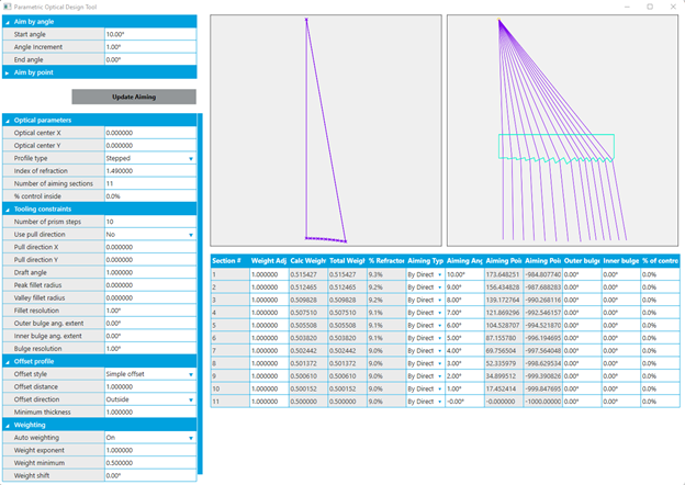
Rhino
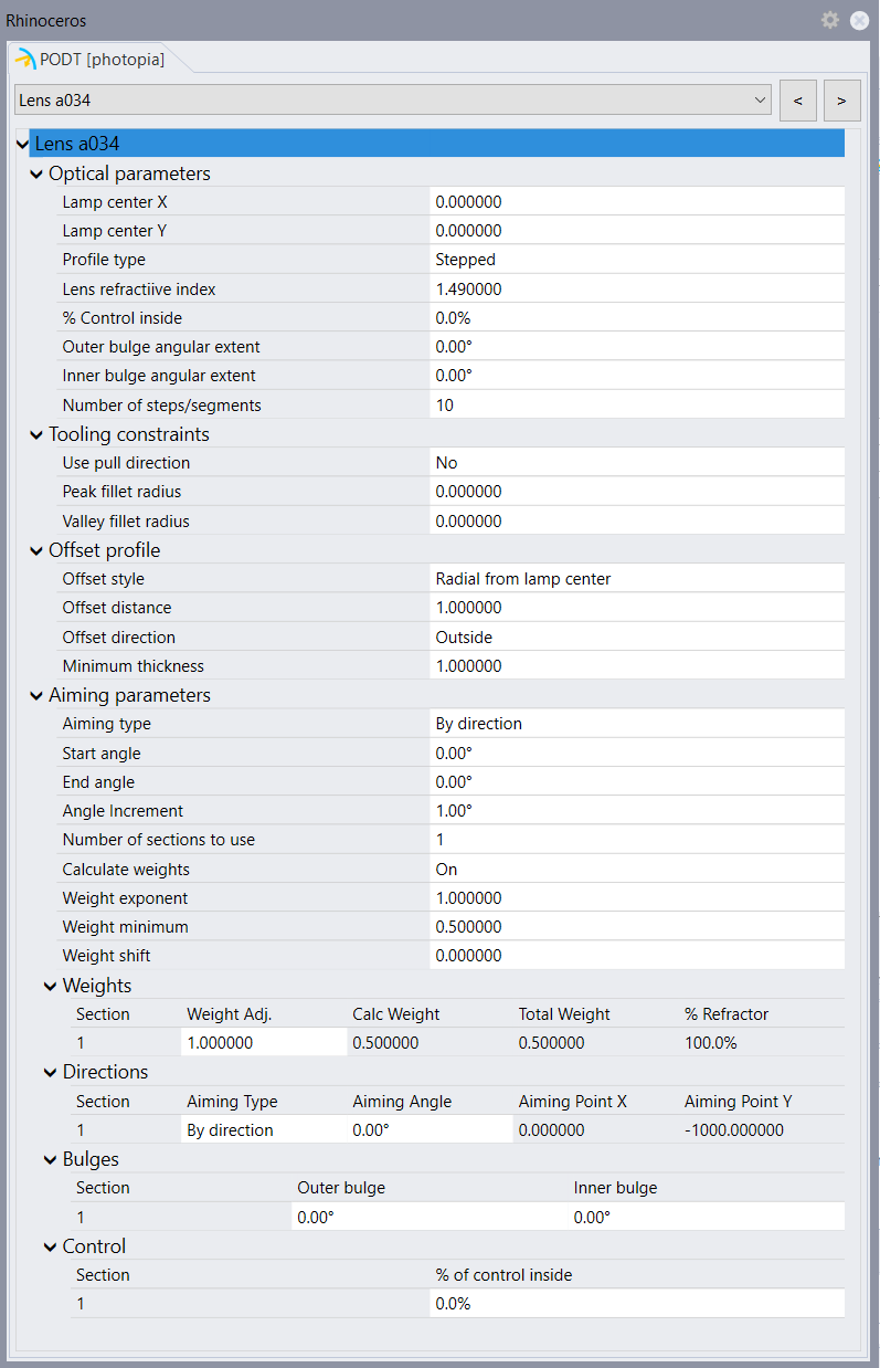
Aim by angle - The aiming angles for the start & end of the base profile as well as the angular increment between the 2 extremes. The start and end points refer to the way the profile was drawn. The angles are measured from the nadir direction. Click "Update Aiming" to apply changes.
Aim by point - The start & end aiming point locations within the sketch/construction plane coordinate system, as well as the number of points in between. The start and end points refer to the way the profile was drawn. Click "Update Aiming" to apply changes.
Optical center X/Y - The focus of all refractor aiming sections in the sketch/construction plane coordinate system.
Profile type - Stepped creates a prismatic lens, Smooth creates a smooth lens. The smooth lens profile is anchored at the “start” of the profile. The smooth lens profile is created by connecting the sloped prism faces together, thus removing the riser steps. Since this adds thickness to the lens, be sure to draw the base profile with the appropriate start point based on which end of the lens profile needs to remain anchored in place.
Index of refraction - The index of refraction used to determine all prism/curvature computations based on the aiming parameters.
Number of aiming sections - The number of aiming sections determined by the aim by angle or aim by point parameters. This value can be overridden if you need to add or subtract sections from what the aiming parameters defined.
% control inside - The final refracted light direction results from light refracting into the inner lens surface and out of the outer lens surface. The initial inner and outer profiles are offset versions of the base profile. Prismatic elements are added to the base profile shape on the inner, outer or both surfaces as defined by this parameter. The images below show the effect of this parameter on a smooth lens profile that connects the prismatic elements together. Note that the start of the base profile was on the right side, which is why that point is fixed in all lens variations.
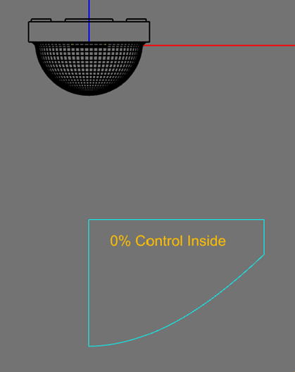
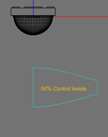
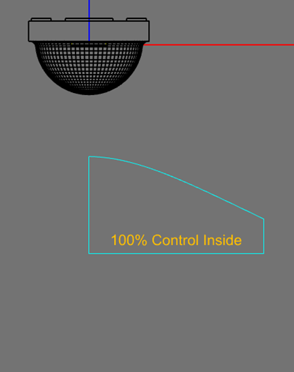
Number of prisms - The minimum number of prisms or steps along a smooth profile. This value is overridden by the # of aiming sections defined since each aiming section requires at least 1 prism or segment along a smooth profile. Use a value higher than the default to create more prismatic features or a smoother smooth lens profile. As seen in some of the prismatic lens images, the size of the prisms may change along the profile. This is a result of keeping all prisms below an internally determined max height. When a prism is determined to go beyond the max height, it is subdivided into 2 prisms. Setting a higher # of prisms can result in a smoother transition in prism sizes along the profile.
Use pull direction - Enables the adjustment of the prism risers based on the tool pull direction vector & draft angle. This parameter is only used for “stepped” (prismatic) profiles. The angle of the risers is oriented along radial lines back to the lamp center by default. This can result in prisms with undercuts on the inner lens surface as shown in the first image below. This is OK for extruded lenses, but not an injection molded lens. The image on the right shows how the prism riser angles change when a vertical pull direction is used.
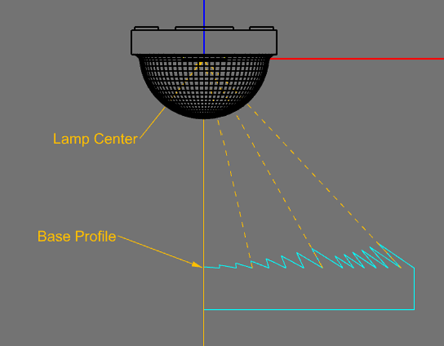
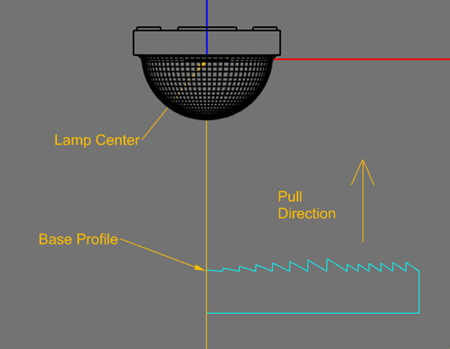
Pull direction X/Y - Defines a direction vector for the pull direction in the sketch/construction plane coordinate system. The image above uses a pull direction X = 0 and Y = 1.
Draft angle - The angle away from the pull direction used to define the prism riser angle.
Peak/Valley fillet radii - The radius of curvature for the fillets used on the peaks & valleys of the prism steps. A value of 0 indicates no fillets will be used, thus all prisms will have sharp peaks & valleys.
Fillet resolution - Fillets are approximated by polyline segments. This parameter defines the angular resolution of the fillet curvature approximation.
Outer/Inner bulge angular extent - Prisms & segments of smooth refractor profiles are flat by default. A “bulge” is an arc shaped curvature added to the flat segment. Bulges create beam spread through each prism/segment. The curvature of a bulge is defined by the angular extent of the arc about the arc center. Thus, the steepest angle away from the flat prism/segment profile is at either end of the arc, with an angle of half the angular extent. See example below that has an angular extent of 40°. For materials with an index near 1.5, light refracts at about half of the profile tilt angle. Therefore, if you want to add 10° of beam spread to either side of the refracted ray directions through your prisms/segments, then enter an angular extent of 40°, 4 times the desired beam spread. The bulge parameters can be defined for the entire optic or individual aiming sections.
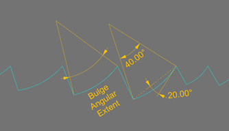
Bulge resolution - Bulge arcs are approximated by polyline segments. This parameter defines the angular resolution of the fillet curvature approximation.
Offset style - The method by which the offset profile is placed. “Simple offset” creates a copy of the base profile perpendicular to the base profile. “Radial from lamp center” creates a scaled version of the base profile along lines from the optical center to the start and end points of the base profile.
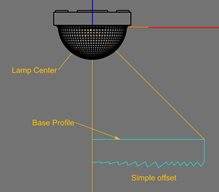
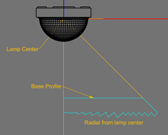
Offset distance - Distance from the base profile start point to the offset profile start point. This is initially set to match the minimum thickness, but may be increased when using a smooth profile and other points along the profile get closer than the minimum thickness to the base profile. Note that this value will not automatically change to find smallest value that meets the minimum thickness requirement as design changes are made. To find the smallest allowable offset distance, enter a value of 0.
Offset direction - Specifies the offset profile direction, to the inside or outside of the base profile.
Minimum thickness - Minimum distance between the inner and outer lens profiles.
Calculate weights - A value of “On” enables the use of the weighting factor (WF) equation.
Weight exponent - Exponent in the WF equation. A higher positive value directs more light toward wider angles. A lower negative value directs more light toward the beam center. A value of 0 sets all WF's to the minimum value.
Weight minimum - Sets a minimum WF value in the nadir (0°) direction.
Weight shift - Shifts the angle in the cosine function of the WF equation. Useful when your beam is directed toward a surface that is not centered about the nadir direction. For example, when illuminating a vertical wall with a ceiling mounted luminaire, using a weight shift of 90° produces a more trend in the WF's.
Weight adjustment -Y An adjustment factor that can be applied to the calculated weights for each aiming section.
TIR Collimator Design Tool Overview
“TIR Collimator” lenses were developed to provide full control of LED light emitted into a single hemisphere. This general lens type is called a “TIR collimator” since the lens features a Total Internal Reflection (TIR) reflecting surface and many initial versions of this type of lens were intended to convert the broad Lambertian emission of an LED into a narrow “collimated” beam. The main features of a TIR collimator lens include an outer profile that reflects light via TIR and a central lens feature that controls light via direct refraction. The basic functionality of a TIR collimator lens is shown in these 2 images:
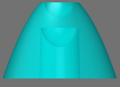
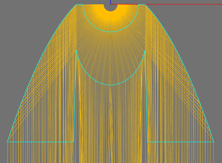
The raytrace shows the inherent advantage of a collimator lens over an open reflector since all rays are controlled, not just the rays captured by the reflector. The TIR surface also reflects with no losses. The TIR surface is important since this allows narrower beams to be created compared to what is possible through direct refraction alone.
Light doesn't need to be aimed toward a single direction with a TIR collimator lens. The TIR reflector surface and central lens feature can aim light toward any desired range of angles.
There are many styles of TIR collimator lenses and Photopia provides 4 to choose from. The one above is called “Outer Shaft” while the “Double Shaft,” “Inner Shaft” and “Stepped” versions are shown below.
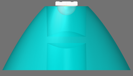
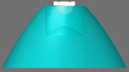
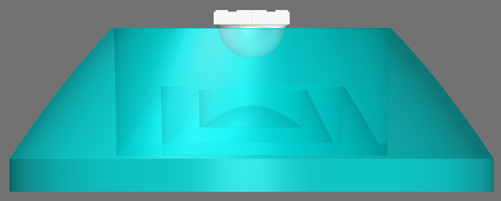
Each collimator style has some advantages and disadvantages, so you choose the best style depending on your design performance priorities and design constraints. Also note that the inner shaft collimator is just a variation of the double shaft collimator. So these 2 styles share the same parameters as described below, but use different default values.
The following images show a range of parameters that can be defined for each of the collimator styles.
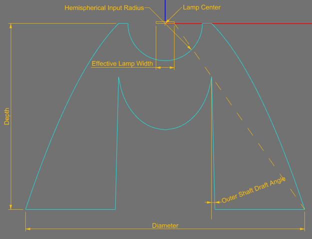
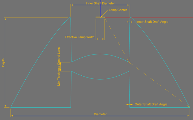
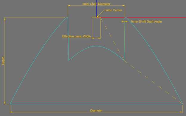
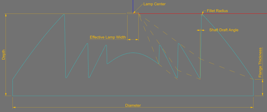
Creating a TIR Collimator
SOLIDWORKS
The TIR Collimator design tool is not yet available inside of Solidworks. Please use Rhino to design TIR collimators.
Rhino
A TIR collimator profile can be created in any construction plane. The Front View is often used when creating a collimator aligned with the default photometric coordinate system. Once you've selected your construction plane, then go to Photopia > Design TIR Collimator on the main menu or click the Design TIR collimator icon on the Photopia toolbar and follow the command prompts for the input parameters. The input parameters are kept to a minimum allowing you to quickly set up a basic collimator lens. More parameters, including the aiming properties, are all defined in the PODT Panel.
Type of collimator - Choose from Outer Shaft, Double Shaft, Inner Shaft and Stepped.
The following input parameters are common to all styles:
Lens Origin - The center of the top opening of the collimator lens.
Lamp Center - The focus of the collimator TIR and central lens aiming sections. This point defaults to the lamp origin, but can be raised above the origin to account for mounting features that may prevent the lamp from being located directly in the center of the top of the lens opening.
Depth - The total depth of the collimator lens.
Diameter - The diameter of the collimator lens, assuming it's revolved. The tool creates the right side lens profile, which you then have the option to revolve or extrude.
Effective lamp width - Refer to the images above to see how this parameter defines the inner or outer shaft depth, depending on the collimator style. The dashed line shows the ray path from the right edge of the “lamp,” which could be a single LED chip, LES of a COB or LED array, to the lower right start point of the TIR profile. In the case of an outer shaft collimator, the line goes straight from the right edge of the lamp to the start of the TIR profile, defining the depth of the outer shaft. In the case of the double and inner shaft collimators, the line goes from the right edge of the lamp to the bottom of the inner shaft, then refracts toward the start of the TIR profile. Designing a collimator with an effective lamp width set to the actual size of the lamp luminous area ensures that all rays emitted from the lamp extent will be reflected by the TIR surface, thus maximizing the optical efficiency. The image below shows how all rays emitting to the left along the extent of the lamp will go toward the TIR surface.
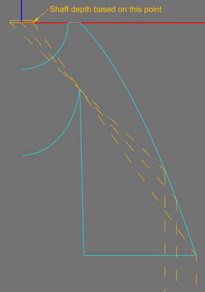
Setting this parameter to 0 causes the shaft depth to be defined by a ray drawn from the optical center. Setting this parameter to a negative value causes the shaft depth to be defined by a ray drawn from the left of the optical center. In all cases where the ray defining the shaft depth is drawn to the left of the actual right edge of the luminous area, some rays emitting to the right of this ray will generally TIR off the flat outer surface and be absorbed in the housing, as illustrated by the red rays in the image below.
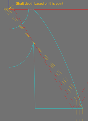
Depending on the collimator dimensions, the red rays could exit out the front flat surface. While this might improve efficiency, those rays would just contribute to stray light outside the main beam. The benefit of moving the start point of the ray defining the shaft depth further to the left is that it moves the central lens feature further from the LED, which reduces the beam spread of light controlled by the central lens. If a design puts a higher priority on a narrower beam angle than the highest possible optical efficiency, then this is a good compromise to consider.
Material Index of refraction - The index of refraction used to determine all prism/curvature computations based on the aiming parameters.
Hemispherical input radius (Outer Shaft) - The radius of the hemispherical input surface.
Minimum lens thickness (Double Shaft) -The minimum thickness of the central lens feature between the inner and outer shafts.
Minimum lens thickness (Inner Shaft) - This parameter is not used in this case, but still prompted for since this is the same tool as the double shaft collimator. Just accept the default value.
Fillet radius (Stepped) - The radius of fillets put onto the peaks & valleys of the TIR feature steps.
Flange thickness (Stepped) - The thickness of the lens between the outer flat surface at the start of the TIR features.
Number of TIR steps (Stepped) - The number of TIR feature steps.
TIR Collimator Window / Dialog
The PODT panel includes some additional parameters, grouped into Optical, Mechanical & Aiming categories.
SOLIDWORKS
Rhino
Exterior refractive index - The default value is 1.0, the value for air. If the collimator lens will be used within a different medium, then the outside index of refraction can be changed to another value. This affects all refracted rays entering and exiting the collimator lens, but does not affect the TIR surface, which always assumes a TIR reaction. Thus, setting this index to a higher value for water, for example, assumes water all around the lens except for the TIR surface, which still assumes an outer medium of air.
TIR curve resolution - Used in conjunction with the TIR profile aiming properties to define the angular resolution of the straight line segments used to construct the TIR profile when the “degree of the curve's spline” is set to 0 or 1 (expert mode required). A value larger than the angular size of each TIR profile aiming section will result in a single line segment for each aiming section.
Number of central lens segments - Used in conjunction with the central lens aiming properties to determine the number of straight line segments used to construct the central lens feature when the “degree of the curve's spline” is set to 0 or 1 (expert mode required).
Percent control inside - (Only for double and inner shaft collimators) When using a double shaft collimator, this allows you to control the percent of the refraction done on the inner and outer surfaces of the central lens feature. Shifting more control to the outer surface can help narrow the beam angle since the angular size of the lamp will be smaller for the lens surface controlling more of the light.
Outer shaft - (Only for double and inner shaft collimators) Included or Hidden. If included, then the percent control on the inside surface can be any value between 0 to 100%. If hidden, then the percent control on the inside surface is forced to 100%.
TIR Collimator Aiming
TIR collimator lenses include separate aiming properties for the TIR profile and central lens features. The aiming parameters are simplified from those available for general parametric reflectors and lenses, with light aimed by angles. The start, end and aiming angle increments are defined for both parts of the collimator. The weighting factor equation values are also defined for both parts of the collimator.
The aiming angles specified for the TIR profile define the “net” aiming desired for light exiting the lens. The TIR profile aiming is automatically adjusted to account for light refracting into and out of the collimator lens.
The image below shows the aiming angle conventions, start points for each feature and the color scheme used to graphically indicate the weighting factor plots for each feature.
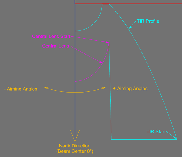
This image shows how the aiming properties are defined for the TIR and central lens features and how their weighting factor plots are displayed in the CAD view, along with their aiming angles.
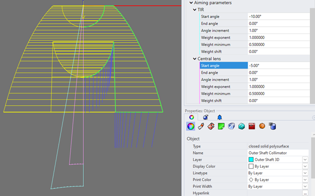
PODT 3D Surface Creation
SOLIDWORKS
The PODT profiles for reflectors and lenses are created in a 2D sketch. 3D features are then created from these sketches using the standard features available in the SW part file. While any type of 3D feature can be created from the sketch containing the PODT profile, Extruded Boss/Base and Revolved Boss/Base features can maintain a direct connection to the PODT parameters and be interactively updated when changes to the PODT parameters are made since they are based on a single PODT profile. Making changes to these types of features as well as any other type of feature is described in the next section on modifying a design.
Rhino
After creating a PODT reflector, lens or TIR collimator in Rhino, a 2D profile is added to the current construction plane. Options to convert the profiles into 3D revolved or extruded surfaces are provided in Photopia's object properties in the Photopia Settings panel. The properties for all Photopia objects in the model are shown in this panel by default. You can isolate the properties for the PODT object you are modifying by selecting it in the CAD view. You may see 2 sets of properties for a PODT object. The first set, identified with the name of the object, shows the PODT surface properties. The second set shown as "Photopia object settings" includes non-PODT properties.
You can create a parametric lofted reflector or lens from a set of PODT profiles using “Loft PODT Profiles” under the Photopia menu or by clicking the PODT Loft icon. This PODT lofting tool provides various symmetry options, allowing you to create complete optical parts with a minimum of profiles. More details are provided in the lofting section below. Lofting is currently not supported for TIR collimator profiles.
You can also parameterize other surface types in Rhino beyond the revolved and extruded options provided in the PODT object by using Rhino's Record History feature. Clicking the Record History button at the bottom of the screen before starting any surface creation tool will create links between the surface and the input geometry. The surface will then automatically be updated whenever you modify the input geometry. The surface maintains Photopia properties such as a material assignment. This allows you to use Photopia PODT profiles as the basis for a much broader range of parametric surfaces such as lofts, sweeps and edge curves. The Record History feature only maintains a single level of parameterization, however. So for example, if you create an extruded surface and later trim that surface, the history will be broken. We have a tutorial for this feature.
Revolved Reflector Surfaces
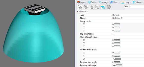
Type - The options are Profile, Revolve & Extrude. This drop down is where you change from a 2D profile to one of the 3D surface types.
Name - Any name you prefer to assign to this object.
Lamp center - The world coordinates of the lamp center (not editable). Editing this location is done in the PODT dialog.
Curve Type - Smooth or segmented.
Flip orientation - Checking this box flips the default orientation of the surface. The default surface orientation is intended to be correct for the raytrace, but it's possible the orientation will not always be correct. See advice below for verifying surface orientations.
Start of revolve axis - The revolve axis start point. The revolve axis defaults to a line through the lamp center in line with the aiming nadir, but can be modified to any location and orientation.
End of revolve axis - The revolve axis end point.
Revolve start angle - The start angle of the revolved surface. 0° is in line with the PODT profile. The default is a full rotation through 360°, but the revolved surface can start and stop at any angle to define partially revolved surfaces.
Revolve end angle - The end angle of the revolved surface.
Extruded Reflector Surfaces
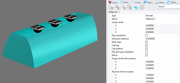
Type - The options are Profile, Revolve & Extrude. This drop down is where you change from a 2D profile to one of the 3D surface types.
Name - Any name you prefer to assign to this object.
Lamp center - The world coordinates of the lamp center (not editable). Editing this location is done in the PODT dialog.
Flip orientation - Checking this box flips the default orientation of the extruded surfaces. The default surface orientation is intended to be correct for the raytrace, but it's possible the orientation will not always be correct. See advice below for verifying surface orientations.
Extrusion Distance - The length of the extrusion away from the profile in a single direction. Values can be positive or negative to extrude in either direction in front or behind the profile location.
Both sides - When checked, this option causes the extrusion distance specified to extend both in front and behind the profile location.
Cap top - Adds and end cap to one end of the extrusion. This is most useful when the extrusion is mirrored as shown in the image above.
Cap bottom - Adds an end cap to the other end of the extrusion.
Flip end cap orientation - Checking this box flips the default orientation of the end cap surfaces. The default surface orientation is intended to be correct for the raytrace, but it's possible the orientation will not always be correct. See advice below for verifying surface orientations.
Mirror - Mirrors the extruded surface about the mirror plane.
Origin of the mirror plane - The location of the mirror plane. The default is at the lamp center.
Normal of the mirror plane - The normal vector of the mirror plane. The default direction orients the mirror plane to be perpendicular to the reflector profile. The mirror plane can be set to any location and any orientation with these 2 parameters.
Revolved Lens Surfaces
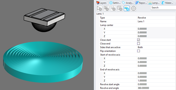
Type - The options are Profile, Revolve & Extrude. This drop down is where you change from a 2D profile to one of the 3D surface types.
Name - Any name you prefer to assign to this object.
Lamp center - The world coordinates of the lamp center (not editable). Editing this location is done in the PODT dialog.
Curve Type - Smooth or segmented.
Close start - When checked, a line segment is included that connects the start point of the base profile to the start point of the offset profile. This line segment is then revolved into a surface unless it is coincident with the revolve axis.
Close end - When checked, a line segment is included that connects the end point of the base profile to the end point of the offset profile. This line segment is then revolved into a surface unless it is coincident with the revolve axis.
Sides that are active - This option allows you to specify which surfaces are included in your model. The options are both, outside only & inside only. This is useful when other surfaces in your model will be used as part of the lens.
Flip orientation - Checking this box flips the default orientation of the surface. The default surface orientation is intended to be correct for the raytrace, but it's possible the orientation will not always be correct. See advice below for verifying surface orientations.
Start of revolve axis - The revolve axis start point. The revolve axis defaults to a line through the lamp center in line with the aiming nadir, but can be modified to any location and orientation.
End of revolve axis - The revolve axis end point.
Revolve start angle - The start angle of the revolved surface. 0° is in line with the PODT profile. The default is a full rotation through 360°, but the revolved surface can start and stop at any angle to define partially revolved surfaces.
Revolve end angle - The end angle of the revolved surface.
Extruded Lens Surfaces
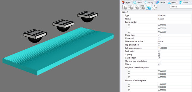
Type - The options are Profile, Revolve & Extrude. This drop down is where you change from a 2D profile to one of the 3D surface types.
Name - Any name you prefer to assign to this object.
Lamp center - The world coordinates of the lamp center (not editable). Editing this location is done in the PODT dialog.
Curve Type - Smooth or segmented.
Flip orientation - Checking this box flips the default orientation of the extruded surfaces. The default surface orientation is intended to be correct for the raytrace, but it's possible the orientation will not always be correct. See advice below for verifying surface orientations.
Close start - When checked, a line segment is included that connects the start point of the base profile to the start point of the offset profile. This line segment is then extruded into a surface unless it is coincident with the mirror plane.
Close end - When checked, a line segment is included that connects the end point of the base profile to the end point of the offset profile. This line segment is then extruded into a surface unless it is coincident with the mirror plane.
Sides that are active - This option allows you to specify which surfaces are included in your model. The options are both, outside only & inside only. This is useful when other surfaces in your model will be used as part of the lens.
Extrusion distance - The length of the extrusion away from the profile in a single direction. Values can be positive or negative to extrude in either direction in front or behind the profile location.
Both sides - When checked, this option causes the extrusion distance specified to extend both in front and behind the profile location.
Cap top - Adds and end cap to one end of the extrusion. This is most useful when the extrusion is mirrored as shown in the image above.
Cap bottom - Adds an end cap to the other end of the extrusion.
Flip end cap orientation - Checking this box flips the default orientation of the end cap surfaces. The default surface orientation is intended to be correct for the raytrace, but it's possible the orientation will not always be correct. See advice below for verifying surface orientations.
Mirror - Mirrors the extruded surface about the mirror plane.
Origin of the mirror plane - The location of the mirror plane. The default is at the lamp center.
Normal of mirror plane - The normal vector of the mirror plane. The default direction orients the mirror plane to be perpendicular to the reflector profile. The mirror plane can be set to any location and any orientation with these 2 parameters.
Revolved TIR Collimator Surfaces
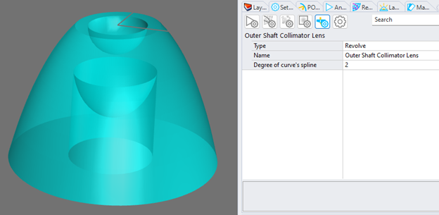
Type - The options are Profile, Revolve & Extrude. This drop down is where you change from a 2D profile to one of the 3D surface types.
Name - Any name you prefer to assign to this object.
Curve Type - Smooth or segmented.
Extruded TIR Collimator Surfaces
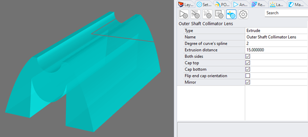
Curve Type - Smooth or segmented.
Extrusion distance – The length of the extrusion away from the profile in a single direction. Values can be positive or negative to extrude in either direction in front or behind the profile location.
Both sides – When checked, this option causes the extrusion distance specified to extend both in front and behind the profile location.
Cap top – Adds and end cap to one end of the extrusion. This is most useful when the extrusion is mirrored as shown in the image above.
Cap bottom – Adds an end cap to the other end of the extrusion.
Flip end cap orientation – Checking this box flips the default orientation of the end cap surfaces. The default surface orientation is intended to be correct for the raytrace, but it’s possible the orientation will not always be correct. See advice below for verifying surface orientations.
Mirror – Mirrors the extruded surface about a default mirror plane through the center of the profile.
Lofted Surfaces
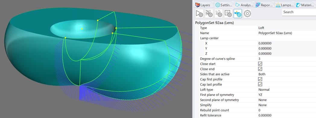
Create a PODT lofted surface by choosing Photopia / Loft PODT Profiles from the main menu or clicking the PODT Loft icon on Photopia’s toolbar. You will be prompted to select the profiles to loft. These can be reflector or lens PODT profile, but all profiles should be of the same type (reflectors and lenses can’t be mixed in a single lofted surface). Select the profiles in the order the surface is to be created. If the optic has symmetry, then be mindful of the order so you can specify the required symmetry planes. The symmetry plane options include XY, XZ, YZ & last profile plane. More than one of these can be selected. When they are specified at the time the loft is created, you are also prompted for a point on the plane, with the origin by default. Press enter at the command line once more after you are finished entering the last symmetry plane origin. Once the lofted surface is created, then all its parameters can be modified in the Photopia object properties panel.
Type - This will be fixed to Loft.
Name - Any name you prefer to assign to this object.
Lamp center - The world coordinates of the lamp center (not editable). Editing this location is done in the PODT dialog for each profile.
Degree of curve’s spline – (Requires enabling expert mode in the general settings.) This defines the smoothness of the surface created through to profiles.
Close start - When checked, a line segment is included that connects the start point of the base profile to the start point of the offset profile. A lofted surface is passed through these line segments unless they are coincident such as when all profiles are rotated around a central axis.
Close end - When checked, a line segment is included that connects the end point of the base profile to the end point of the offset profile. A lofted surface is passed through these line segments unless they are coincident.
Sides that are active - This option allows you to specify which surfaces are included in your model. The options are both, outside only & inside only. This is useful when other surfaces in your model will be used as part of the lens.
Cap first profile – If the lofted surface does not fully enclose itself, then this option creates a flat surface over the first PODT profile.
Cap last profile – If the lofted surface does not fully enclose itself, then this option creates a flat surface over the last PODT profile.
Loft type – This defines how the NURBS surface is created from the profiles.
>Normal - The surface has an average amount of stretching between the curves. This is the default and a good choice when the curves are proceeding in a relatively straight path or there is a lot of space between the curves.
Tight - The surface closely follows the original. This is a good choice when the input curves are going around a corner.
Straight - Creates a ruled surface. The sections between the curves are straight.
Uniform - Makes the object knot vectors uniform.
First plane of symmetry – The symmetry plane options include XY, XZ, YZ & Last profile plane. The “Last profile plane” option is useful when you require symmetry about a non-orthogonal plane. An example is a square beam optic that is based on 2 profiles, one along the XZ plane and the other along a diagonal plane. Using the “Last profile plane,” YZ and XZ, in that order, creates the complete optic with “octalateral” symmetry.
Second plane of symmetry… – Multiple symmetry planes can be specified, but each plane option can only be selected once. So the choice of planes only includes options not already selected.
Simplify – (Requires enabling expert mode in the general settings.) This option relates to the PODT cross-section curve profiles. The options are:
None - Do not simplify. The curves will not be rebuilt.
Rebuild - Rebuild the shape of the curves with the specified number of control points before lofting.
Refit - Refits the shape of the curves to the specified tolerance value before lofting.
Both sides - When checked, this option causes the extrusion distance specified to extend both in front and behind the profile location.
Cap top - Adds and end cap to one end of the extrusion. This is most useful when the extrusion is mirrored as shown in the image above.
Cap bottom - Adds an end cap to the other end of the extrusion.
Flip end cap orientation - Checking this box flips the default orientation of the end cap surfaces. The default surface orientation is intended to be correct for the raytrace, but it’s possible the orientation will not always be correct. See advice below for verifying surface orientations.
Mirror - Mirrors the extruded surface about the mirror plane.
Origin of the mirror plane - The location of the mirror plane. The default is at the lamp center.
Normal of mirror plane - The normal vector of the mirror plane. The default direction orients the mirror plane to be perpendicular to the reflector profile. The mirror plane can be set to any location and any orientation with these 2 parameters.
Surface Orientation
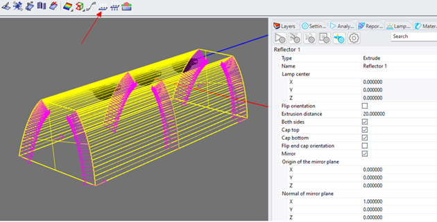
The 3D surfaces created by Photopia are intended to be properly oriented for the raytracer, but are not guaranteed to always be correct. So it’s best to use Rhino’s "Show Object Direction" tool on the Surface Tools panel with the icon indicated above to confirm the surface orientations. If they are not properly oriented, then use the Flip orientation parameter to reverse their direction. It’s best to use Photopia’s flip orientation parameter so the surface orientation is properly maintained as you change other PODT surface parameters. Reflector surface normals should face toward the lamp. Lens surface normals should face to the outside of the lens geometry.
PODT Object Coordinate System
PODT geometric parameters are generally relative to a local PODT object coordinate system. This coordinate system is indicated with 3 lines anchored to the lamp center point, as shown in the image below. The long solid line indicates the local X-axis, the shorter solid line indicates the local Y-axis and the arrow indicates the aiming nadir direction. For TIR collimators, the depth and diameter dimensions are relative to this coordinate system, even if the object has been moved and rotated from its original position. Aiming angles are relative to the arrow direction.
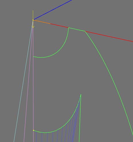
Modifying a Design
SOLIDWORKS
If you create an Extruded Boss/Base or a Revolved Boss/Base feature from your PODT profile, then you can then select that feature in the FeatureManager, then choose Photopia > Design Reflector/Lens. If this is the first time you are editing this feature, then click the drop-down list under Reload and select the reference to the properties you had previously defined. These properties will now be associated with this feature. You'll see the feature name referenced under Target Feature. The next time you edit the optical properties of this feature, you can directly click the button to open the PODT window. When finished, close the PODT window, then click the check on the PropertyManager page. The profile will be regenerated in the sketch and the feature will be updated with the new sketch geometry.
If you use multiple PODT profiles to create other types of features such as a Swept, Lofted or Boundary Boss/Base, then edit the sketch with the PODT profile you want to modify. Then choose Photopia > Design Reflector/Lens and Reload the latest reference to the PODT parameters for this particular sketch. Using named PODT profiles is most helpful in this case and be sure to check the option to Clear Sketch Contours. Once the parameters are loaded, then click the button to open the PODT window. Make the desired changes and close that window, then click the check on the PropertyManagment page. Once the sketch is closed, then the associated feature will be updated with the new sketch geometry.
If you create an Extruded Boss/Base or a Revolved Boss/Base feature from your PODT profile, then you can then select that feature in the FeatureManager, then choose Photopia > Design Reflector/Lens. If this is the first time you are editing this feature, then click the drop-down list under Reload and select the reference to the properties you had previously defined. These properties will now be associated with this feature. You’ll see the feature name referenced under Target Feature. The next time you edit the optical properties of this feature, you can directly click the button to open the PODT window. When finished, close the PODT window, then click the check on the PropertyManager page. The profile will be regenerated in the sketch and the feature will be updated with the new sketch geometry
If you use the PODT profile to create another feature type (surfaces, lofted, swept, etc.) our add-in will not automatically replace the profile in the feature, but you can still generate a new PODT profile and manually replace the reference in your feature.
Rhino
Select the PODT profile or surface in the CAD view. If you want to edit the profile parameters, click on the “Design reflector” or “Design lens” icon. This will open the PODT dialog. Changes will be shown in the CAD view once the dialog is closed.
If you want to change surface parameters, then open the Photopia object properties in the Photopia Settings panel.
PODT lofted surfaces maintain an internal copy of the original PODT profiles from which they were created. To modify the profiles of the lofted surface, you therefore need to select the lofted surface, then click on the “Design reflector” or “Design lens” icon. You will be prompted at the command line for the profile number to modify. The profiles are numbered in the order they were selected, starting at 0. You need to close the PODT profile window and click the icon to open it again to select a new profile to modify. The original profiles will still be in your model, but selecting and modifying them will not affect the lofted surface.
Spherical Lens Tool
Photopia supports smooth spherical lens parts when created with the Spherical lens feature. The raytracer will treat the lens geometry as mathematically smooth (not meshed) surfaces. The part definitions support convex, concave, and flat surfaces on each side of the lens, as well as annulus features. Using spherical lens parts allows Photopia to better support a range of applications including luminous images, lasers, LIDAR, machine vision, and basic imaging analyses.
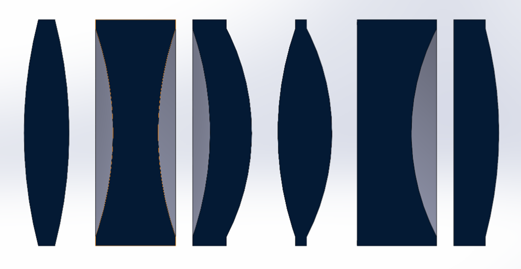
Create a Spherical Lens
SOLIDWORKS
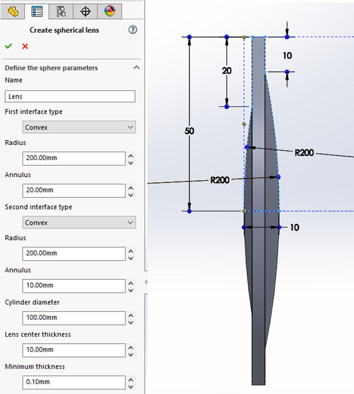
Open a new part file and start a new sketch in any plane you prefer. The profile of the lens will be constructed in this sketch plane. Click the “Spherical lens” icon. This part is used solely to define a Photopia spherical lens object and no other features should be added. The lens is defined with the following parameters:
Name -Any name you choose as a description for the lens.
Interface type for each lens surface -Specify convex, concave or plane.
Radius for each lens surface -The radius of curvature of the spherical surface is specified in the part model units.
Annulus for each lens surface -The width of a flat flange feature on the lens. This can be unique on each side of the lens.
Cylinder diameter -The overall lens diameter, including the annulus features.
Lens center thickness -The total thickness through the lens center. The value entered will be overridden if any part of the lens gets smaller than the specified minimum thickness. Enter 0 for the lens to be constructed as thin as possible.
Minimum thickness -The minimum thickness of any part of the lens construction. This will be at the outer circumference if the lens is convex on both sides but can be in the lens center if either side is concave.
Rhino
The spherical lens tool is coming soon to Rhino.
Modifying a Spherical Lens
SOLIDWORKS
After a lens is defined, you can modify the lens parameters by selecting the Revolve feature in the part file, then clicking on the “Spherical lens” icon.
Rhino
The spherical lens tool is coming soon to Rhino.
Placing a Spherical Lens
SOLIDWORKS
You can place the spherical lens part just like any other part file using standard mates to any of the solid part geometry or reference planes. The lens part can also be patterned like any other part in an assembly.
Rhino
The spherical lens tool is coming soon to Rhino.
Limitations for Spherical Lenses
SOLIDWORKS
The lens parts are limited to round/revolved shapes and do not support additional features in the same part file.
A single Photopia appearance should be assigned to the entire part as Photopia does not support appearance assignment by face on smooth spherical lens parts.
A single spherical lens part feature is required in a single lens part file.
Rhino
The spherical lens tool is coming soon to Rhino.
Weighting Factors
When the goal of the optical design is to achieve a specific intensity distribution, you need to define both the directions over which the light is aimed as well as the amount of light aimed toward each direction. The aiming parameters defined for reflectors and lenses cover the former. Weighting factors cover the latter.
The weighting factors (WF's) indicate the relative importance/size of each aiming section of the optical profile. The way the WF's work is illustrated in the reflector profile image below. Each reflector section is aimed toward a unique angle in the beam and is assigned a relative WF value. The absolute magnitude of the WF's isn't important, only their relative values with respect to each other. The fraction of the reflector Angular Extent that is allocated toward each aiming section is determined by dividing the WF for that section by the total of all WF's.
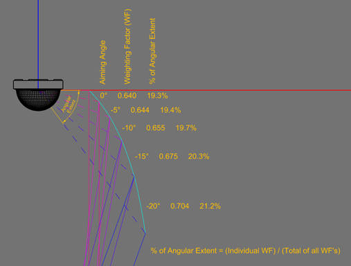
The value of this system is that it allows for quick relative changes to your design by changing a single value. For example, if you need more light at the widest aiming angle, then you simply increase that WF. That aiming section increases in size, while all the rest proportionally shrink. The example above shows higher WF values at the wider aiming angles. These result in a higher fraction of the angular extent allocated to the wider aiming angles.
The rules apply in the same way to lens optics. In their case, the angular extent is the full angle subtended by the Base Profile about the lamp center. The angular extent determined for each aiming section based on their WF's is then projected onto the base profile.
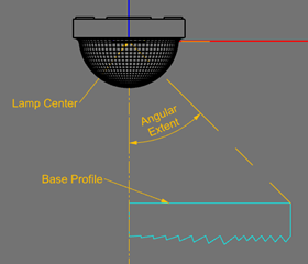
Weighting Factor Equation
Smoothly changing beams are often required for many applications. These are generally achieved with smoothly changing WF’s, which result in smoothly changing optical profile geometry.
Although WF’s can be entered manually, Photopia provides a WF equation that creates useful trends of smoothly changing WF’s over the entire distribution. For example, if you need to produce even illuminance/irradiance values over a surface below your optic, then you will need an increasing intensity at wider beam angles. This requires WF’s that increase at a user defined rate as a function of the angle away from the beam center. Conversely, if you require a narrower beam optic with the peak in the beam center, fading to a desired beam angle, then you need WF’s that peak at the beam center and decrease at a user defined rate at the wider beam angles. The WF equation has parameters that allow for these types of distributions and more. Understanding the WF equation is important since it allows you to make desired changes to your entire set of WF’s by changing a single parameter of the equation.
The core of the WF equation is:
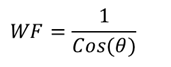
Where ϴ is the angle in your intensity distribution. We chose this starting point for the equation since it has the trend of increasing WF’s at wider beam angles, a commonly desired beam trend. The following images show a quick review of the cosine function. It’s the x-component of the radius of a circle as it rotates counter-clockwise from the X-axis. It starts at 1.0 at ϴ=0°, the beam center, and drops to 0 at ϴ=90°.
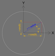
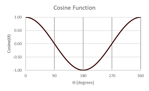
So the inverse of the cosine function increases non-linearly as ϴ goes from 0° to 90°. Since the equation divides by 0 at ϴ=90°, the WF value is capped to a maximum of 100.
To add more flexibility to this equation, such as defining the rate at which the WF’s increase at wider angles, an exponent n was added to the cosine function:
As n increases, the WF increases at a faster rate at the wider beam angles, thus more light is directed toward the wider beam angles and less toward the beam center. This results in intensity distributions with trends such as this.
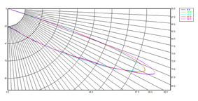
If a negative exponent is entered, then the equation inverts so that the highest WF is at ϴ=0°. Decreasing n to lower negative values causes a greater emphasis of the WF in the beam center. Negative n values create beams with trends like this.
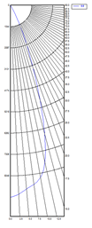
Two more parameters were added to the WF equation that allow you to explicitly define the value at ϴ=0° and rotate the frame of reference when illuminating surfaces that aren’t horizontal below your optic. The WF 1.0 equation adds some absolute values to avoid negative WF values. The WF 2.0 equation doesn’t apply any absolute values and simply sets the WF to 0 if the equation produces a negative value. This works well to automatically remove wider aiming angles as the exponent goes to lower negative values, which is common when designing a narrower beam angle. The WF 1.0 equation was the default through V2023 while WF 2.0 is the default from V2024 forward. The final equations are shown here:
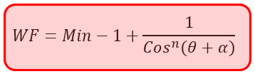
Where:
WF = weighting factor
ϴ = angle in the distribution
n = Weight exponent
Min = Weight minimum (defines the WF at ϴ=0°)
α = Weight shift (angular shift in cosine function)
While it’s best to define your entire set of WF’s with the equation whenever possible, there are times when you need to manually adjust WF’s in specific parts of the beam. Multipliers are therefore provided for each aiming section of your optic.
Scripting & Optimization
SOLIDWORKS
Advanced Scripting and Optimization are currently only avaliable in Photopia for Rhino. All users of Photopia for Solidworks have access to Photopia for Rhino as well. If you don't own a seat of Rhino, you can purchase that from LTI Optics directly.
Rhino
Overview
All Photopia commands in Rhino can be run in scripts. Scripts are files that list a series of commands to be run automatically. Scripts can also include programming logic, such as running loops & comparing the values of variables. There are multiple scripting language options in Rhino, but this section focuses on the use of PythonScript.
In addition to scripting, Rhino also includes a visual programming language (VPL) called Grasshopper (GH). GH allows you to build geometry interactively/parametrically, using a wide range of geometry creation tools/components. Several tutorials that use GH “definitions” are shown on our Rhino tutorials page.
All Photopia PODT profile parameters can be obtained and set via the PhotopiaGet and PhotopiaSet commands. Most any output parameter can also be obtained via the PhotopiaEvalImmediate command. Since these and all other Photopia commands can be scripted, this provides Photopia for Rhino with the ability to run automated sets of simulations for tasks such as tolerancing and design optimizations.
For example, you can set up a revolved parametric reflector that needs to produce a specific beam angle. Starting with your specified reflector aiming angles, the beam angle will be a function of the weighting factor (WF) distribution. More specifically, the WF exponent. Since the known performance trend is that a higher WF exponent produces a wider beam angle, a script can be written that prompts for the desired beam angle, then runs a set of raytraces while progressively changing the WF exponent until the desired beam angle is reached.
Designs reach their desired result faster when parameter changes have a known effect on performance, as in the previous example. Optimization processes can also be run where a larger number of parameters are varied, but those will take much longer since many more design variations need to be evaluated. In these cases, there are benefits to using methods such as genetic algorithms that narrow in on solutions based on the success of previous iterations. This type of optimization can be done using the Galapagos evolutionary solver in GH.
We have provided some example Python scripts and GH definitions that pursue specific types of design optimizations. While these are useful on their own, they also provide helpful references for developing your own optimization tools. Modifying the examples requires some programming knowledge, so the following sections provide a range of references to help you get started developing your own optimization tools.
Opening, Editing and Running a Python Script
To open and edit, go to the Rhino main menu and choose Tools > PythonScript > Edit.... Browse to the location of the .py file you want to open.
To run a python script, click the Run button while the script is open. You can also choose Tools > PythonScript > Run....
Photopia Commands for Scripting
The following commands can be run via the RhinoScript “Command” function, which is available within Python scripts. The example below shows how the “PhotopiaRaytraceSettings” command is run with 2 input values. The “i” is passed to the command to choose the “Initial source rays” option. The “numRaysCourse” variable fills in the curly brackets { } placeholder with a value.

You can manually run these commands in Rhino to see all their argument options. Note that the “!” preceding the command name in the example above cancels any previous command that might be running, the “_” references the English version of the command no matter your Rhino language setting and the “-“ suppresses a dialog box if one
https://docs.mcneel.com/rhino/7/help/en-us/information/rhinoscripting.htm
A few of these commands are intended to set or return values based on variables in the script, which isn’t a standard feature of Rhino commands. More information is provided for these commands below as they are used in a special way in a Python script.
PhotopiaAddLamp
PhotopiaAnisotropicOrientation
PhotopiaEval
PhotopiaEvalImmediate – This command returns a value when passed one of the evaluation expressions described in the Photopia Evaluation Expressions section below. An “evaluation expression” is basically an output variable name, but the full “expression” can also include mathematical operations and comparisons operators. When used in a Python script, the value is assigned to a program variable in the script via the document user text. So this is best done in a function, as shown below and in some of the example scripts.
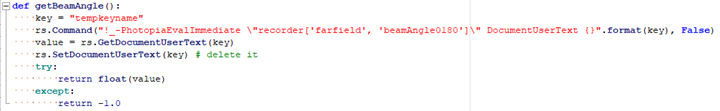
PhotopiaGet – This command returns a value when passed one of the PODT property names listed in the following section.
PhotopiaImport
PhotopiaInsertBlock
PhotopiaLoftedPODT
PhotopiaMaterial – The material filename prefix is passed to this command along with the material type identifier, as shown in the example below. This example also defines the entire material string can be defined as a variable, which is then passed to the command in the .format function. The material filenames can be seen in the material list under the “Library Name” column. The type identifiers include (reflective), (transmissive) & (refractive). When this command is run in a script, then material will be assigned to the currently selected geometry.

PhotopiaMeshParameters
PhotopiaOut – Exports a range of file types from the Photopia model, including the full Raytrace Results Data (RRD) file, a Photopia Job Data (PJD) file and the intensity distribution as an IES or LDT file. The code example below selects the IES file option with the “i” value, and then provides a filename. If the full path is not provided, then the file is exported to the location of the active 3DM file.

PhotopiaPODTLens
PhotopiaPODTReflector
PhotopiaPurge
PhotopiaRaytrace
PhotopiaRaytraceCancel
PhotopiaRaytraceSettings
PhotopiaRealizeRays
PhotopiaRecordingPlane
PhotopiaSelection
PhotopiaSet – This command sets a value when passed one of the PODT property names listed in the following section along with the value to be set. To simplify the syntax of setting PODT parameter values in a Python script, it’s best to define a function as shown in the sample scripts.

PhotopiaView
PhotopiaGet & PhotopiaSet Property Names
The PODT profile property names listed below can be obtained and set via the PhotopiaGet and PhotopiaSet commands. The case sensitive property names should be passed into these commands exactly as the bolded strings are shown. The set of values with a number in square brackets are repeated for each aiming section of the optical profile. The value in the brackets indicates the aiming section number, beginning with 1. All distance/dimension values are in the current model units and in the construction plane of optical profile. All angle values are in degrees.[Aiming parameters]Aiming type - Options are “By direction” or “By point.”
[Aiming parameters]Start angle - The start aiming angle to be used in the aiming script if the aiming type is “By direction.”
[Aiming parameters]End angle - The end aiming angle to be used in the aiming script if the aiming type is “By direction.”
[Aiming parameters]Angle Increment - The aiming angle increment to be used in the aiming script if the aiming type is “By direction.”
[Aiming parameters]Start point X - The start aiming point X value to be used in the aiming script if the aiming type is “By point.”
[Aiming parameters]Start point Y - The start aiming point Y value to be used in the aiming script if the aiming type is “By point.”
[Aiming parameters]End point X - The end aiming point X value to be used in the aiming script if the aiming type is “By point.”
[Aiming parameters]End point Y - The end aiming point Y value to be used in the aiming script if the aiming type is “By point.”
[Aiming parameters]Number of sections - The number of aiming sections to be used in the aiming script if the aiming type is “By point.”
[Aiming parameters]Weight exponent - The weighing factor exponent.
[Aiming parameters]Weight minimum - The weighting factor in the beam center.
[Aiming parameters]Weight shift - The angular shift used in the weighting factor equation.
[Optical parameters]Optical center X - X value for the optical center/focus.
[Optical parameters]Optical center Y - X value for the optical center/focus.
[Optical parameters]Curve resolution - The angular resolution of the polyline approximation for the reflector aiming sections.
[Optical parameters]Lens refractive index - Lens index of refraction, e.g., 1.491 for pmma.
[Optical parameters]Number of steps/segments - Number of aiming sections. This value is automatically determined based on the range of aiming angles or aiming points.
[Optical parameters]% Control inside - Percentage of the refractive control on the inside surface for the entire lens, e.g. 50 = 50%.
[Optical parameters]Outer bulge ang. extent - The angular extent of the outer bulge for the entire lens.
[Optical parameters]Inner bulge ang. extent - The angular extent of the inner bulge for the entire lens.
[Mechanical parameters]Start X - X value of the reflector start point.
[Mechanical parameters]Start Y - Y value of the reflector start point.
[Mechanical parameters]Angular extent - The angular extent of the reflector, sweeping around the optical center. Counterclockwise is positive.
[Tooling constraints]Use pull direction - Options are “Yes” or “No.”
[Tooling constraints]Pull direction X - Tool pull direction X-direction vector value.
[Tooling constraints]Pull direction Y - Tool pull direction Y-direction vector value.
[Tooling constraints]Draft angle - Draft angle value in degrees.
[Tooling constraints]Peak fillet radius - The fillet radius of curvature for the peaks of prismatic lens elements.
[Tooling constraints]Valley fillet radius - The fillet radius of curvature for the valleys of prismatic lens elements.
[Offset profile]Offset style - Options are “Radial from lamp center” and “Simple offset.”
[Offset profile]Offset distance - Distance to the start of the of the offset lens profile.
[Offset profile]Offset direction - Options are “Outside” or “Inside.”
[Offset profile]Minimum thickness - The minimum distance between the inner and outer lens profiles.
Curve type - Options are “Smooth” or “Stepped.”
[Weights][1]Weight Adj. - Weighting factor adjustment value for aiming section 1. Value must be greater than or equal to 0.
[Directions][1]Aiming Type - Options are “By direction” or “By point.”
[Directions][1]Aiming Angle - The aiming angle to be used if the aiming type is “By direction.”
[Directions][1]Aiming Point X - The aiming point X value to be used if the aiming type is “By point.”
[Directions][1]Aiming Point Y - The aiming point Y value to be used if the aiming type is “By point.”
[Bulge][1]Outer bulge - The angular extent of the outer bulge for aiming section 1.
[Bulge][1]Inner bulge - The angular extent of the inner bulge for aiming section 1.
[Control][1]% of control inside - Percentage of the refractive control on the inside surface for aiming section 1, e.g. 50 = 50%.
Photopia Evaluation Expressions
The Photopia evaluation expressions, or output value property names, are passed to the PhotopiaEvalImmediate command to return the values into a Python script. The expression strings should exactly match the names shown in the Photopia Evaluation panel. To see all expression options, first enable the view of the Evaluation (photopia) panel:
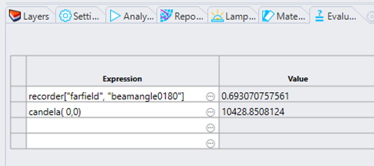
Then click the “…” icon in one of the Expression boxes. This will open a dialog with all available evaluation expressions. The list is large, so you can use the search box to help find specific output values.
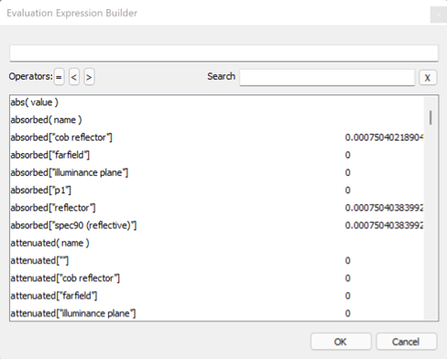
A few example property names are:
candela( phi, theta ) - An individual intensity value at the specified phi (horizontal) and theta (vertical) angles, given in degrees.
recorder["farfield", "beamangle0180"] - The beam angle in degrees, in the 0-180° plane.
recorder["farfield", "beamangle90270"] - The beam angle in degrees, in the 90-270° plane.
recorder['farfield', 'maxintensity'] - The maximum intensity value in the full distribution.
recorder['farfield', 'maxintensityh'] - The horizontal angle in degrees, at which the maximum intensity value was achieved.
recorder['farfield', 'maxintensityv'] - The vertical angle in degrees, at which the maximum intensity value was achieved.
Optimization with Galapagos
The Galapagos genetic optimization engine is a component you select from the Util section of the Params panel inside of Grasshopper. Its icon is circled in red below:
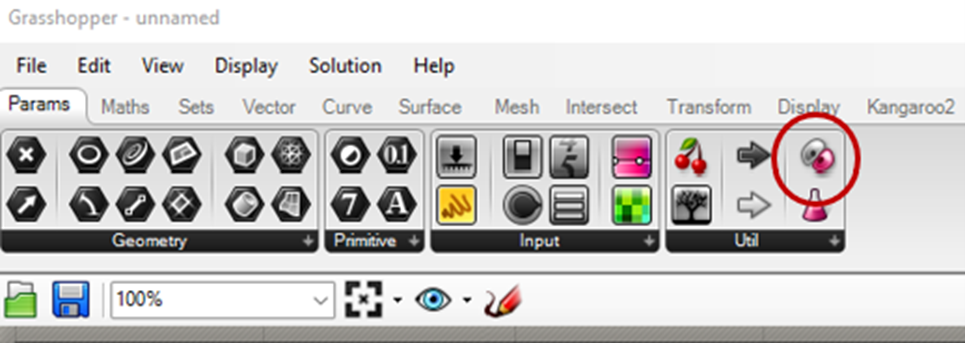
The Galapagos component allows you to connect any number of input variables with their ranges defined on slider bars. These define your “Genome” or the range of options to be explored. A single “Fitness” variable is also defined. The PODT reflector design example below shows input values of the WF exponent, the start aiming angle and the end aiming angle as the genome. The fitness value is the difference between the desired beam angle and the beam angle achieved by the current reflector being tested. In this case, the optimization seeks a fitness value of 0.

The Galapagos component randomly changes the values on the slider bars one at a time. Each change causes the Python module to modify a PODT reflector and then run a raytrace with that reflector. The output of the Python script module is the difference between the beam angle goal and the beam angle produced by the current reflector. Settings within the Galapagos editor allow you to define the number of design iterations for each “generation” of the design. For example, if you choose 50 iterations, then 50 random variations of the input variables will be run. Once that generation of simulations is complete, then new design variations will be selected for the next generation guided by the best results from the previous generation. The next generation will also include some fraction of design options that are more random and not based on the previous best results. Settings for all these types of generation parameters are defined in the Galapagos editor. As multiple generations of design variations are run, the design generally tends toward the optimal desired result, as shown in the upper left plot below for 10 generations.
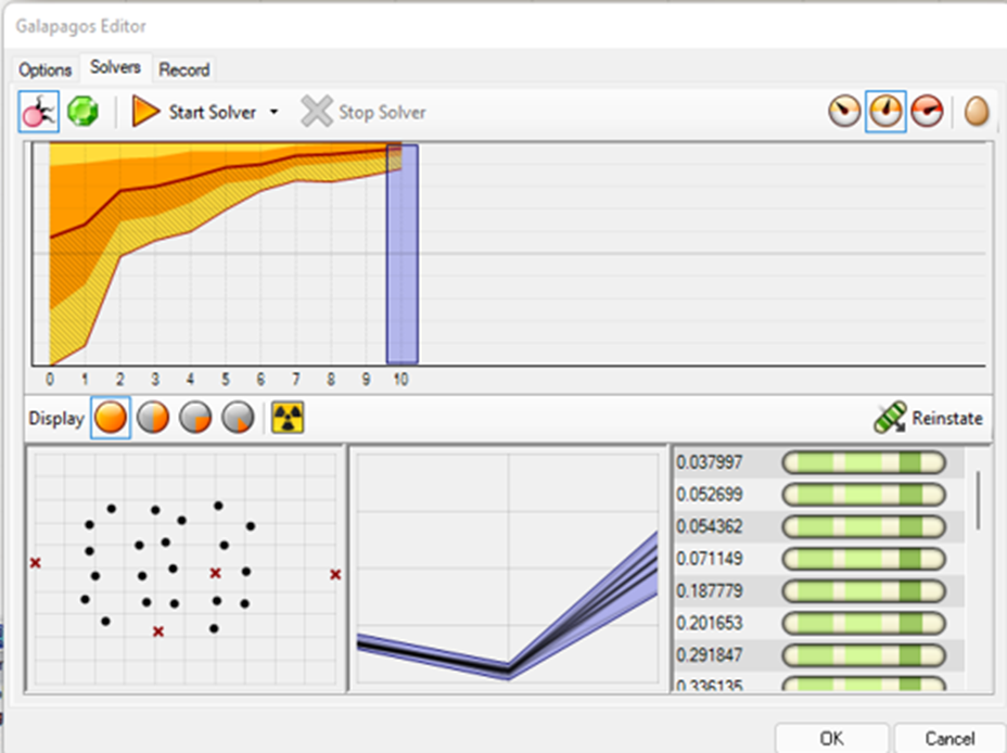
See more information about Galapagos in the tutorials on this page:
https://grasshopperdocs.com/addons/galapagos.html
Other References
Rhino's Python References: https://developer.rhino3d.com/guides/rhinopython/
Rhino's General API References: https://developer.rhino3d.com/api/
Rhino Scripting: https://docs.mcneel.com/rhino/7/help/en-us/information/rhinoscripting.htm
Galapagos Information: https://grasshopperdocs.com/addons/galapagos.html
More Python Scripting Language Documentation: https://www.w3schools.com/python/default.asp
McNeel's Grasshopper Intro and Tutorials: https://www.rhino3d.com/learn/?query=kind:%20grasshopper&modal=null
More Grasshopper Intro and Tutorials: https://thedifferentdesign.com
- Create a free account if you don't already have one.
- Go to "Computation & Analysis Courses" and choose "Grasshopper for Beginners."
- We recommend watching videos 01, 02 & 08 and any others of interest.
- More videos are available with a subscription to this website.
General Settings
SOLIDWORKS
Choose Tools > Photopia > General Settings to display the Photopia Settings PropertyManagement page.
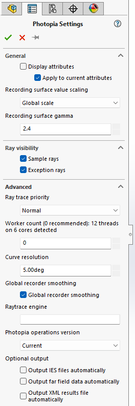
Display attributes - All Photopia data associated with the model is stored as attributes. References to these attributes is generally hidden in the FeatureManager but can be viewed by checking this option. Photopia attributes are indicated with a symbol and text describing the type of data, like "PhotopiaSettings". Deleting specific attributes will remove that data from the model, but this should be done only with a clear knowledge of the data being removed.
Recording surface value scaling & gamma - These parameters are generally set in the Recording surface settings PropertyManagement page and may be removed from these options in the future.
Ray visibility - Allows you to indicate the types of rays displayed in the CAD view. Sample rays are standard rays from the ray trace while exception rays are those from any of anomalous interactions.
Ray trace priority - The options are normal, high & aggressive. Using normal will keep your computer most responsive when performing other tasks while a ray trace is running.
Worker count - This defines the # of processor cores that will be used by the ray tracer. Leaving the value at 0 is generally recommended since then Photopia will use the # of cores reported by the operating system. If you know your total # of physical & logical cores, then you can enter that value explicitly or use a value lower than the total to maintain more responsiveness on your computer while running a ray trace. If you have multiple physical processors, then it's best to manually enter the total # of physical & logical cores on both processors here, since Windows generally only reports the total # of cores on a single processor.
Curve resolution - The angular resolution of polyline approximations of arcs used in PODT lens base profiles & fillets.
Global recording smoothing - This parameter is generally set in the Recording surface settings PropertyManagement page and may be removed from these options in the future.
Raytrace engine - A blank value indicates the current ray trace engine is being used. A different version can be entered here if ever required.
Photopia operations version - This relates to a range of functionality for running ray traces and processing output. We recommend keeping this value set to “Current.” If there is ever a need to use an earlier version, then any previously installed version can be selected here.
Optional output - Checking these files will cause them to be automatically written when the raytrace is run. The filenames will share the same name and be written to the same folder as your assembly model.
IES file - The IESNA LM-63 standard format file containing the intensity distribution data. Double clicking on this file will open Photopia Reports, allowing you to view photometric reports and intensity distribution plots. No recorder report data will be available in Reports, however.
Farfield data dump - The far field data dump (*.ffdd) file is an ASCII file that contains the raw data from which the intensity distribution & color data is obtained. The first line in the space delimited file indicates the values in each column. Note that the flux values are always in radiant watts regardless of your lamp flux energy units setting. SPD data will be 0’s when running in tristimulus mode. This data file is useful when performing your own data processing on the far field photometric sphere data.
XML results file - The Raytrace Results Data (*.RRD) file is an XML based file that contains all intensity distribution data, recorder data & raytrace report related data. All formatted reports are created from the data in this file. Double clicking on this file will open Photopia Reports, allowing you to view any reports or plots. This file can also be read by any custom data processing tools built by us or yourself.
Rhino
Choose Tools > Options to display the Rhino Options window and then click on Photopia in the navigation pane.
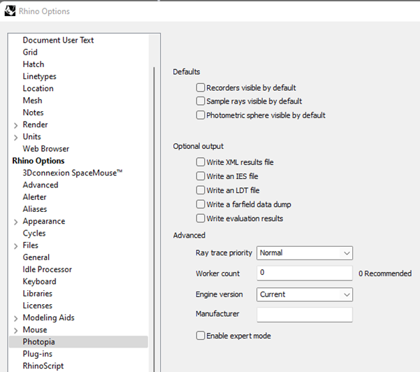
Defaults - Set the default visibility of recorders, sample rays & the photometric sphere. Each of these items can be toggled on & off via their icons on the Photopia toolbar.
Optional output - Checking these files will cause them to be automatically written when the raytrace is run. The filenames will share the same prefix and be written to the same folder as the Rhino model.
XML results file - The Raytrace Results Data (*.RRD) file is an XML based file that contains all intensity distribution data, recorder data & raytrace report related data. All formatted reports are created from the data in this file. Double clicking on this file will open Photopia Reports, allowing you to view any reports or plots. This file can also be read by any custom data processing tools built by us or yourself.
IES file - The IESNA LM-63 standard format file containing the intensity distribution data. Double clicking on this file will open Photopia Reports, allowing you to view photometric reports and intensity distribution plots. No recorder report data will be available in Reports, however.
LDT file - The EULUMDAT “standard” format photometric file containing the intensity distribution data. Double clicking on this file will open Photopia Reports, allowing you to view photometric reports and intensity plots. No recorder report data will be available in Reports, however.
Farfield data dump - The far field data dump (*.ffdd) file is an ASCII file that contains the raw data from which the intensity distribution & color data is obtained. The first line in the space delimited file indicates the values in each column. Note that the flux values are always in radiant watts regardless of your lamp flux energy units setting. SPD data will be 0’s when running in tristimulus mode. This data file is useful when performing your own data processing on the far field photometric sphere data.
Evaluation results - The raw data available to Photopia’s evaluation system, which is used to test a large range of output values against any requirements you define. The *.evalresults file is XML based and can be read by any custom data processing tools built by us or yourself.
Ray trace priority - The options are normal, high & aggressive. Using normal will keep your computer most responsive when performing other tasks while a ray trace is running.
Worker count - This defines the # of processor cores that will be used by the ray tracer. Leaving the value at 0 is generally recommended since then Photopia will use the # of cores reported by the operating system. If you know your total # of physical & logical cores, then you can enter that value explicitly or use a value lower than the total to maintain more responsiveness on your computer while running a ray trace.If you have multiple physical processors, then it's best to manually enter the total # of physical & logical cores on both processors here, since Windows generally only reports the total # of cores on a single processor.
Engine version - We recommend keeping this value set to “Current.” If there is ever a need to use an earlier version of the ray trace engine, then any previously installed version can be selected here.
Manufacturer - Enter your company name here if you want it specified within the IES file.
Enable expert mode - This option enables extra features in the plug-in interface that generally require a deeper understanding of the software to properly use. Currently, the only extra feature it enables is some additional checks on importing lamp models.